When analyzing data in Excel, it’s not always enough to find the overall maximum value. In real-world scenarios, you often need to apply conditions like identifying the highest sales for a specific team, region, or both. Whether you’re managing marketing performance, comparing regional sales, or tracking departmental results, Excel offers flexible ways to find the maximum value that meets one or more conditions.
In this article, we’ll learn how to find the maximum value in Excel based on one or multiple conditions using functions like MAX, IF, MAXIFS, SUMPRODUCT, and AGGREGATE. Each method includes step-by-step instructions and uses a sample dataset so you can follow along easily.
Steps to find the maximum value in Excel with Condition:
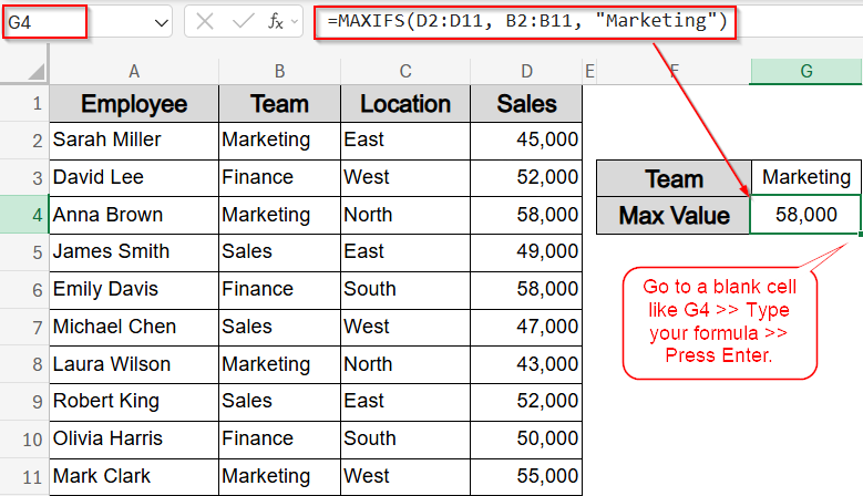
➤ Select a blank cell like G4.
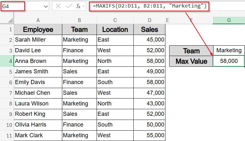
➤ To find highest sales in Marketing team, type this formula:
=MAXIFS(D2:D11, B2:B11, “Marketing”)
➤ Press Enter to display output.
Find Max Value with Single or Multiple Conditions Using Max and IF Functions
When working with filtered data, you might want to find the highest value based on one or more conditions like identifying the top salary in the Sales department, or the highest amount from a specific region and team. This method uses the IF function with MAX to apply logic-based filtering and return the correct maximum. It’s useful for conditional analysis when your dataset includes categories like Team and Location.
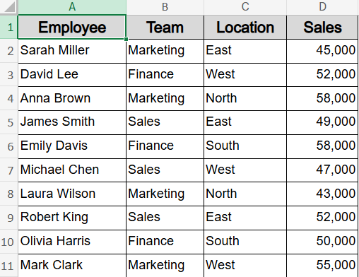
To demonstrate each method clearly, we’ll use a consistent dataset containing sales records for ten employees. The table includes columns for Employee, Team, Location, and Sales. This setup allows us to apply both single and multiple conditions like finding the highest Sales in a specific Team, Location, or a combination of both.
Steps:
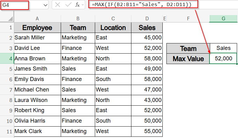
➤ Select a blank cell like G4.
➤ Enter this array formula to find the max salary for Sales department:
=MAX(IF(B2:B11=”Sales”, D2:D11))
➤ Press Ctrl + Shift + Enter in older Excel and just Enter in Excel 365.
➤ For multiple conditions, use this formula to find max value from Sales department in the East region:
=MAX(IF((B2:B11=”Sales”)*(C2:C11=”East”), D2:D11))
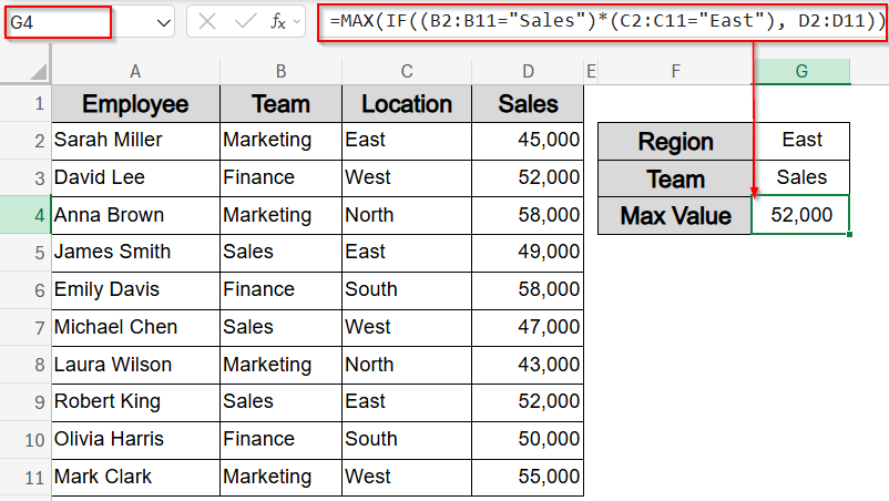
Now you have filtered your data based on multiple criteria to derive the maximum sales value which is 52,000.
Apply MAXIFS Function for Conditional Maximum (Excel 2019 and later)
The MAXIFS function is the simplest and most direct way to find the maximum value based on one or more conditions without needing array formulas or nested logic. It’s especially useful when working in Excel 2019 or Excel 365. In this method, we’ll use it to extract the highest Sales value from specific Team and Location criteria.
Steps:
➤ Select a blank cell like G4.
➤ To find highest sales in Marketing team, type this formula:
=MAXIFS(D2:D11, B2:B11, “Marketing”)
➤ Press Enter.
➤ For multiple criteria such as Sales team from East region, use this formula in G4 cell:
=MAXIFS(D2:D11, B2:B11, “Sales”, C2:C11, “East”)
➤ Press Enter to display output.
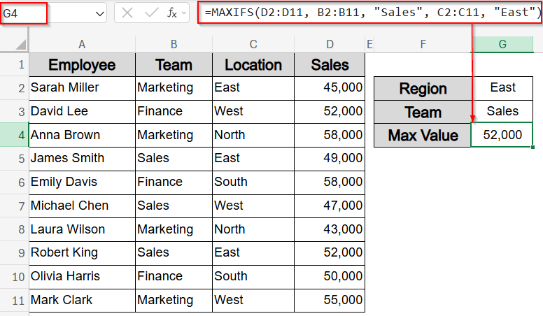
This returns the respective maximum sales value based on set criteria such as Region and Team.
Use SUMPRODUCT Function for Conditional Maximum Calculation
The SUMPRODUCT function allows for conditional max calculations even in Excel versions that don’t support MAXIFS. It multiplies logical arrays to isolate values that meet all your conditions, then returns the highest one. This method is ideal when working with older Excel versions and delivers a clean output showing the top value based on multiple filters. We will find the highest Sales value from the Marketing team and East region in this method.
Steps:
➤ Select a blank cell like G4.
➤ To find max sales for Marketing team in East location, enter formula:
=SUMPRODUCT(MAX((B2:B11=”Marketing”)*(C2:C11=”East”)*D2:D11))
➤ Press Ctrl + Shift + Enter if necessary.
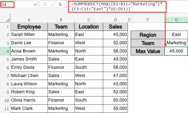
Now the highest sales value meeting your conditions appears instantly from the dataset which is 45,000 without needing helper columns or advanced functions.
Use AGGREGATE Function with Division Logic for Conditional Maximum Value
The AGGREGATE function is a flexible tool that returns the maximum value while automatically ignoring hidden rows or errors. When combined with division logic, it can evaluate specific conditions and extract the filtered maximum. In our example dataset, this method helps retrieve the highest sales figure within a specific team, such as “Marketing“, while keeping the formula short and dynamic.
Steps:
➤ Select a blank cell like G4.
➤ To find max sales in Marketing team:
=AGGREGATE(14, 6, D2:D11/(B2:B11=”Marketing”), 1)
➤ Press Enter.
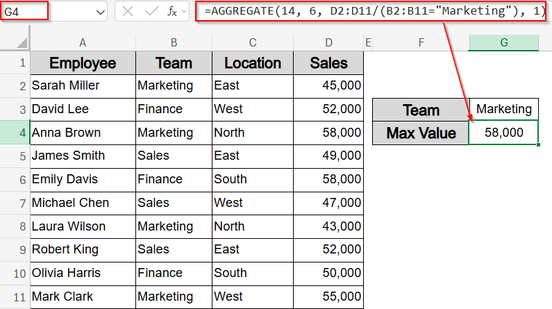
Now you’ll get the highest Sales value (58,000) in the Marketing team based on your condition, while any errors or hidden rows in the range will be ignored neatly.
Retrieve Associated Data Using INDEX and MATCH Functions
Once you’ve identified the maximum value based on conditions, you might want to return related information such as the employee’s name tied to that max value. The combination of INDEX and MATCH functions allow you to locate this associated data dynamically. This approach works especially well when paired with conditional max formulas like MAXIFS.
In this example, we will find the employee name that has the maximum Sales value from the Marketing team.
Steps:
➤ Select a blank cell like G4.
➤ To find the employee with the highest sales in Marketing department, type this formula:
=INDEX(A2:A11, MATCH(MAXIFS(D2:D11, B2:B11, “Marketing”), D2:D11, 0))
➤ Press Enter.
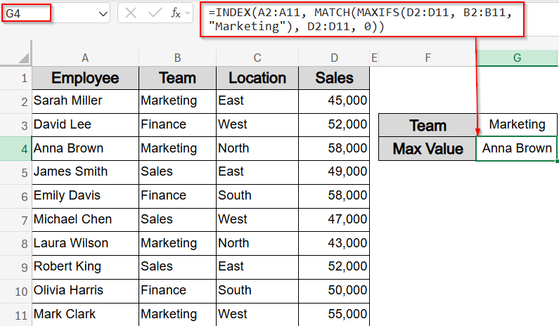
This returns the name of the employee Anna Brown having the highest sales of 58,000 from the Marketing team.
Try MAX/SUMPRODUCT Function with OR Logic for Multiple Criteria
When you need to find the highest value based on any of multiple conditions, for example, top sales made by either the Marketing or Sales team in a specific region, Excel doesn’t provide a direct OR function inside MAXIFS. Instead, using MAX or SUMPRODUCT function with OR logic (+ operator or curly braces) helps compare multiple groups at once. This approach returns the highest value meeting either of the given conditions, not necessarily both.
Let’s apply this logic to find the maximum sales made by either Marketing or Sales teams in the West region. The result will pinpoint the top qualifying sales figure based on flexible OR-based filtering.
Steps:
➤ Select a blank cell like G4.
➤ Enter this formula to find the max sales for either Marketing or Sales team in the West region:
=MAX((B2:B11={“Marketing”,”Sales”})*(C2:C11=”West”)*D2:D11)
➤ Press Ctrl + Shift + Enter in older Excel, or just Enter in Excel 365.
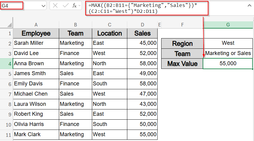
This returns the maximum sales value which is 55,000 matching either of the Team and the Region condition.
➤ Alternatively, use this formula in older Excel versions without needing array entries:
=SUMPRODUCT(MAX(((B2:B11=”Marketing”) + (C2:C11=”East”)) * D2:D11))
➤ Press Enter.
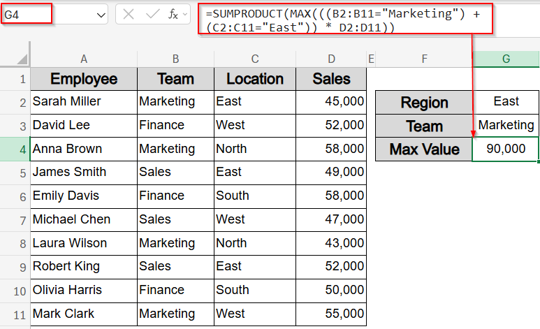
This returns the highest sales figure where the team is either Marketing or the region is East.
Use MAXIFS for Multiple Dynamic Criteria (Excel 2019 and Later)
When your conditions change based on user input like selecting a team and region from dropdowns MAXIFS function works perfectly with cell-based criteria. This method lets you pull the highest value that meets both dynamic filters without updating the formula each time. It’s ideal for interactive dashboards or models with flexible inputs.
For example, if G2 contains “South” and G3 contains “Finance”, the formula will return the highest sales value from that specific combination.
Steps:
➤ Suppose G2 contains “South” and G3 contains “Finance” as your criteria.
➤ Select a blank cell like G4.
➤ Type this formula:
=MAXIFS(D2:D11, B2:B11, G3, C2:C11, G2)
➤ Press Enter.
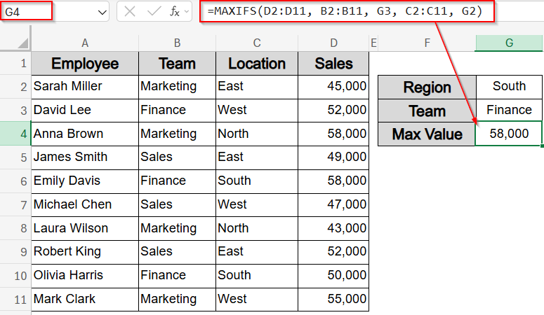
This returns the maximum value from the Sales column for rows where Team equals Finance and Region equals South.
Frequently Asked Questions
Can I use MAXIFS for multiple conditions in Excel?
Yes, MAXIFS function supports multiple conditions by pairing each criteria range with its corresponding condition. It’s a built-in function in Excel 2019 and later, requiring no array formulas.
What Excel versions support the MAXIFS function?
MAXIFS function is available in Excel 2019, Excel 365, and later versions. Users of earlier versions must use alternatives like MAX + IF or SUMPRODUCT function with array formulas to achieve similar results.
How do I return names tied to the max value?
Use INDEX and MATCH alongside MAXIFS function or other max logic formulas. This allows you to pull associated data like employee names linked to the maximum value found in your dataset.
Can I find max values based on OR logic in criteria?
Yes, SUMPRODUCT and array formulas can handle OR logic by using addition between conditions. For example, (Team=”Sales”)+(Team=”Marketing”) filters both conditions before applying the MAX or MAXIFS function.
Wrapping Up
In this tutorial, we learned how to find the maximum value in Excel with one or more conditions using functions like MAX, MAXIFS, SUMPRODUCT, and AGGREGATE. Each method suits different Excel versions and levels of complexity. Choose the one that fits your dataset and version best. Feel free to download the practice file and share your feedback.