
When working with spreadsheets, you may often need to count how many values in a column are not equal to a specific text, like how many employees haven’t said “Yes” or how many responses differ from “No.” In Google Sheets, you can achieve this using the COUNTIF function in combination with logical operators like <>.
In this article, we’ll walk you through step-by-step methods to count values not equal to specific text using your sample data. We’ll also include variations like excluding blanks, handling multiple conditions, using cell references, and wildcard usage.
Steps to count cells not equal to specific text in Google Sheets:
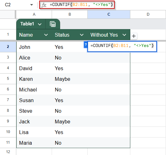
➤ Click on any blank cell (e.g., C2)
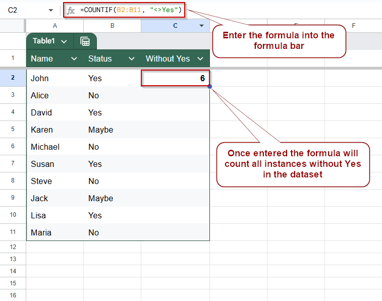
➤ Enter this formula: =COUNTIF(B2:B11, “<>Yes”)
➤ Press Enter.
Count Cells Not Equal to Specific Text
This method helps you count how many cells in a range do not contain a specific word or value. For instance, if you’re tracking responses in a “Yes/No” column and want to count how many entries are not “Yes”, this approach is ideal. It’s useful in surveys, attendance logs, and status trackers where you need to isolate non-matching entries.
This is the dataset we will use to demonstrate all the methods in this article. In this method, we will count the number of instances where the entries are “Yes”.
➤ Click on any blank cell (e.g., C2)
➤ Enter this formula:
=COUNTIF(B2:B11, “<>Yes”)
➤ Press Enter.
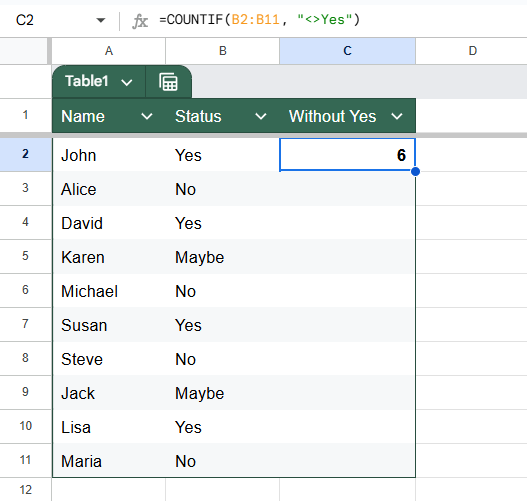
This counts all the entries in the Status column that are not exactly “Yes”.
In this dataset, it will return 6 because there are 4 “No” and 2 “Maybe”.
Use a Cell Reference Instead of Hardcoded Text in COUNTIF in Google Sheets
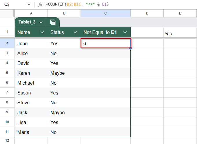
When you want to make your formula flexible and easy to update, it’s best to avoid hardcoding the text you’re comparing against. Instead, you can use a cell reference to control what value should be excluded dynamically. This is especially helpful in cases where the criteria might change, for example, switching between “Yes”, “No”, or “Pending”, without needing to edit the formula each time.
Let’s say you’re tracking responses or statuses in column B, and you want to count how many are not equal to a certain value entered in another cell (like E1). This method will update the count automatically whenever the reference cell changes.
➤ In cell E1, type the word Yes.
➤ In any other cell, use this formula:
=COUNTIF(B2:B11, “<>” & E1)
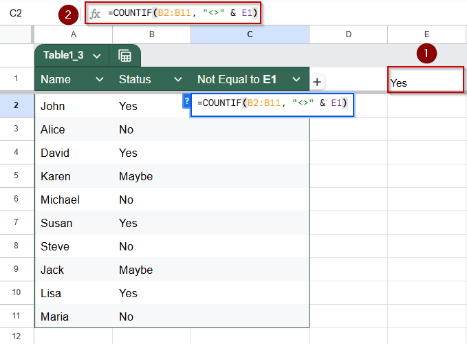
➤ Press Enter.
Count Cells Not Equal to Multiple Text Values in Google Sheets
When analyzing data in Google Sheets, you may need to count how many cells exclude multiple specific values, for example, cells that are neither “Yes” nor “No”. This method is especially helpful when working with survey responses, status fields, or any dataset where you want to isolate “other” or non-standard entries like “Maybe”, “N/A”, or blanks.
Google Sheets doesn’t support a direct “NOT IN” condition like SQL, but you can use the COUNTIFS function to layer multiple exclusion conditions.
Steps:
➤ Click on a blank cell where you want the result (e.g., C2)
➤ Enter the formula:
=COUNTIFS(B2:B11, “<>Yes”, B2:B11, “<>No”)
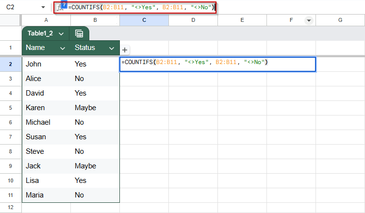
➤ Press Enter
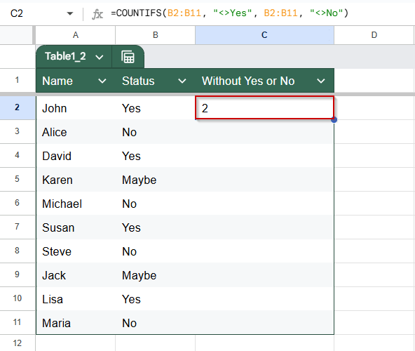
The formula will return a count of all cells in B2:B11 that are not equal to “Yes” and also not equal to “No”. For example, if “Maybe” is the only alternative in the list, it will return 2 if “Maybe” appears twice.
Exclude Blanks While Counting Cells Not Equal to a Specific Text in Google Sheets
When analyzing responses or tracking data in Google Sheets, it’s common to encounter blank cells. Suppose you’re counting how many cells don’t contain a specific word (like “Yes”). In that case, you might not want to include those blanks in your results, especially if empty cells represent unsubmitted or irrelevant entries.
By combining COUNTIF with COUNTBLANK, you can accurately count only the non-blank cells that don’t match a specific value.
Steps:
➤ Click on a blank cell where you want to display the count (e.g., C2)
➤ Enter the formula:
=COUNTIF(B2:B11, “<>Yes”) – COUNTBLANK(B2:B11)
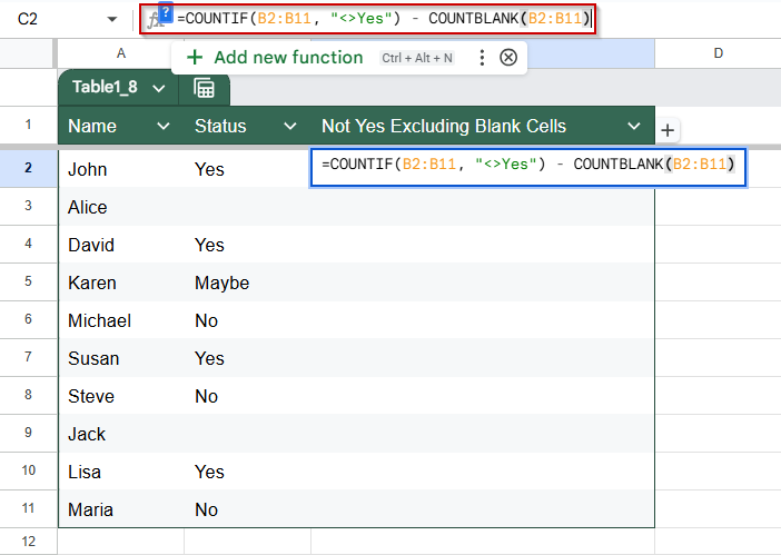
➤ Press Enter
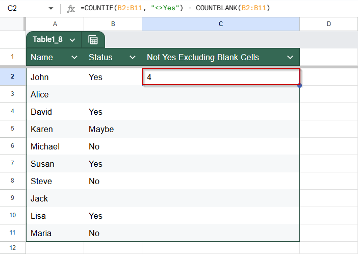
This returns the number of cells in B2:B11 that are not equal to “Yes”, excluding any that are blank. This ensures your count reflects only meaningful, non-empty data.
Use ARRAYFORMULA with FILTER Function for Larger Ranges
When working with larger or dynamic datasets in Google Sheets, ARRAYFORMULA allows your formulas to adapt automatically as new data is added. By combining it with FILTER, you can count all values in a column that do not match a specific word, like “Yes”, while maintaining flexibility and performance.
This method is useful when the dataset size changes frequently, and you want a formula that doesn’t require constant updating.
Steps:
➤ Click on a blank cell where you want the result to appear (e.g., C2)
➤ Enter the following formula:
=COUNTA(FILTER(B2:B11, B2:B11 <> “Yes”))
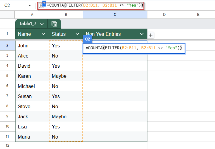
➤ Press Enter

➧ COUNTA function then counts those filtered, non-Yes.
This combination gives you a dynamic and efficient count of all non-“Yes” cells, adapting automatically as the range grows.
Frequently Asked Questions
Can COUNTIF be used for not equal comparisons in Google Sheets?
Yes. Use the <> operator within the criteria string, like “<>” & “Yes”.
Will COUNTIF ignore blank cells?
No. You need to exclude blanks manually using COUNTIFS or subtracting COUNTBLANK.
Can I use wildcards in COUNTIF with not equal?
Yes, but you must use “<>” along with *, such as “<>*Yes*”.
How do I count cells not equal to multiple values?
Use COUNTIFS with both conditions. For three or more exclusions, use an array or FILTER+COUNTA.
Wrapping Up
Using COUNTIF with the <> operator in Google Sheets gives you precise control over how you count data that doesn’t match a specific text. Whether you’re comparing a single condition, handling blanks, or managing multiple exclusions, the step-by-step methods here should cover everything you need.


I need help… haha
I have a column that contains 2 letter state codes. I want a count of state codes of everything BUT AL, GA, TN and blanks.
I can’t seem to get this figured out.
You can do this using COUNTIFS with multiple “not equal to” criteria. If your state codes are in column A, use:
=COUNTIFS(A:A, "<>AL", A:A, "<>GA", A:A, "<>TN", A:A, "<>")Explanation:
“< >AL” excludes AL
“< >GA” excludes GA
“< >TN” excludes TN
“< >” excludes blank cells
This will count all state codes except AL, GA, TN, and blanks. If you run into any issues, make sure there are no extra spaces in the cells (you can use TRIM if needed).