When working with large datasets in Google Sheets, apply the VLOOKUP function across an entire column without manually dragging the formula down. Unfortunately, Google Sheets does not apply VLOOKUP to entire arrays by default. However, combining it with ARRAYFORMULA provides an efficient solution.
This article walks you through how to use ARRAYFORMULA with VLOOKUP to automatically retrieve data for multiple rows, without repetitive manual entry.
Steps to use ARRAYFORMULA with VLOOKUP
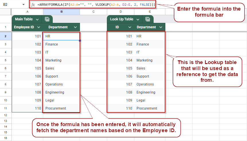
➤ Select the cell where you want your results to begin (e.g., B2).
➤ Enter the following formula:
=ARRAYFORMULA(IF(A2:A=””, “”, VLOOKUP(A2:A, D2:E, 2, FALSE)))
➤ Press Enter.
ARRAYFORMULA with VLOOKUP to Lookup Across Multiple Rows in Google Sheets
When managing datasets where each row requires a lookup, such as assigning departments to employee IDs or retrieving product details based on SKUs, manually copying VLOOKUP down each row can be inefficient and error-prone. Google Sheets’ ARRAYFORMULA function allows you to apply a formula to an entire column dynamically, eliminating the need for repeated manual entry.
By combining ARRAYFORMULA with VLOOKUP, you can automatically populate multiple rows at once based on a lookup table, saving time and keeping your sheet clean and responsive.
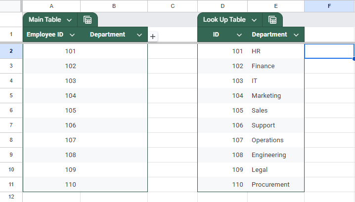
This is the dataset that we will be using to demonstrate the method:
Steps:
➤ Select the cell where you want your results to begin (e.g., B2).
➤ Enter the following formula:
=ARRAYFORMULA(IF(A2:A=””, “”, VLOOKUP(A2:A, D2:E, 2, FALSE)))
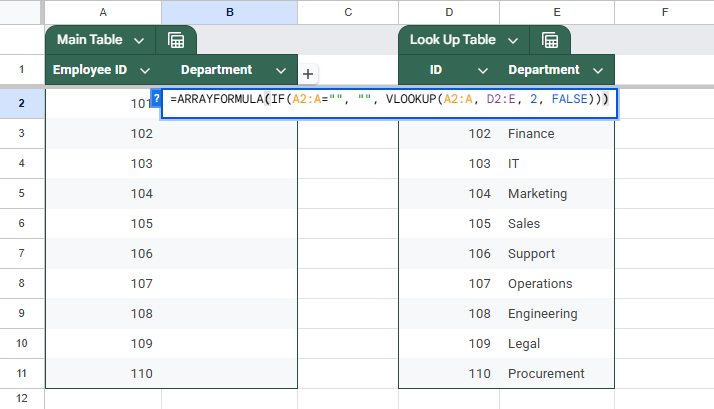
➤ Press Enter.
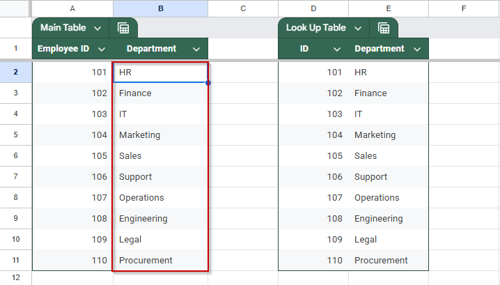
This will automatically populate column B with department names matching the IDs in column A.
Combining UNIQUE Function to Return Distinct Lookup Results
When working with datasets that include repeated values, such as employee IDs referencing the same department, you may want to perform a lookup that returns each matching value only once. Google Sheets allows you to do this by combining the UNIQUE, ARRAYFORMULA, and VLOOKUP functions.
Steps:
➤ Select the cell where you want the unique lookup results to begin (e.g., B2 or another column).
➤ Enter the following formula:
=UNIQUE(ARRAYFORMULA(IF(A2:A=””, “”, VLOOKUP(A2:A, D2:E, 2, FALSE))))

➤ Press Enter.
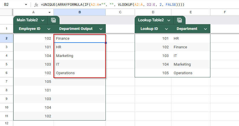
This will return a list of department names corresponding to the employee IDs in column A, with duplicate departments removed.
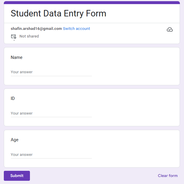
Merge Google Forms Responses into a Summary Sheet
When collecting responses through Google Forms, the linked Google Sheet automatically captures new entries in real time. However, if you need to create a clean, separate summary sheet, perhaps showing names, emails, or answers in a different format, you can use ARRAYFORMULA with VLOOKUP to dynamically pull and update the data.
This method allows you to reference the original response data and automatically fill in values on another sheet, eliminating the need to re-enter or manually drag formulas.
This is the sample form we are using for this method:
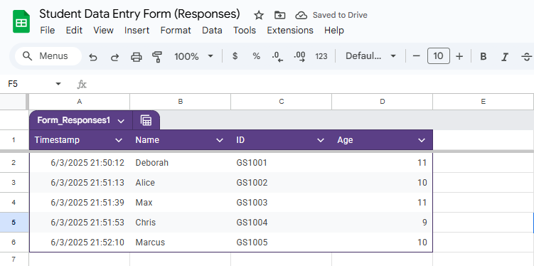
This is the response sheet linked to the form:
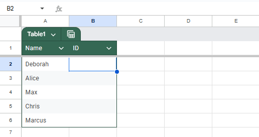
This is the summary sheet that we will be using:
Steps:
➤ In the Summary Sheet, select cell B2 (next to the first name).
➤ Enter the following formula:
=ARRAYFORMULA(IF(A2:A=””, “”, VLOOKUP(A2:A, ‘Form Responses 1’!B:C, 2, FALSE)))
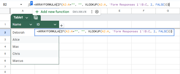
➤ Press Enter.
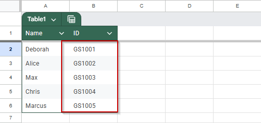
➥ Return the corresponding email from column C.
➥ Automatically apply the logic to every row in the list.
As new names are added to the Summary Sheet, the email field will populate automatically, assuming those names exist in the Form Responses.
Frequently Asked Questions
Can I use this method if the lookup table (columns D and E) is on a different sheet?
Yes, you can. Just reference the other sheet by name in the formula. For example: =UNIQUE(ARRAYFORMULA(IF(A2:A=””, “”, VLOOKUP(A2:A, Sheet2!D2:E, 2, FALSE))))
What happens if a value in column A doesn’t exist in the lookup table?
If an ID from column A isn’t found in the lookup table, the formula will return a #N/A error for that entry. You can wrap the VLOOKUP in IFERROR to handle this:
=UNIQUE(ARRAYFORMULA(IF(A2:A=””, “”, IFERROR(VLOOKUP(A2:A, D2:E, 2, FALSE), “Not Found”))))
Does the UNIQUE function remove blank cells from the result?
Yes, UNIQUE automatically filters out blank values in its output, so your result will only contain actual department names.
Will this update automatically if I change the values in the lookup table?
Yes, this formula is dynamic. If you update the data in columns A or D:E, the result will refresh automatically with the new lookup matches and updated unique values.
Wrapping Up
Using ARRAYFORMULA with VLOOKUP in Google Sheets enables you to perform lookups across entire columns without manually duplicating formulas. When combined with UNIQUE, it can also return a distinct list of results, ideal for summaries and validation ranges. This approach ensures your sheet remains dynamic and scalable, making it useful when dealing with frequently changing data or large datasets.