If your Google Sheets formula isn’t working, it can disrupt your entire workflow. Whether you’re seeing errors, blank results, or unexpected outputs, the issue often comes down to syntax errors, data types, incorrect cell references, or formatting problems. Understanding the root cause helps you troubleshoot and fix the issue faster.
In this article, we will guide you through the most common reasons a formula might fail in Google Sheets, providing simple and actionable steps to resolve them.
Steps to fix common formula errors in Google Sheets:
➤ Use correct syntax and formula structure
➤ Check for missing equal signs (=)
➤ Make sure your data types match (text vs. number)
➤ Remove hidden characters using CLEAN or TRIM
➤ Verify that cell references and ranges are accurate
Start with an Equal Sign and Check for Typing Errors
One of the most common reasons a formula does not work in Google Sheets is due to simple input errors. Forgetting to begin the formula with an equal sign, using incorrect function names, or misplacing punctuation can all cause the formula to fail or display as plain text.
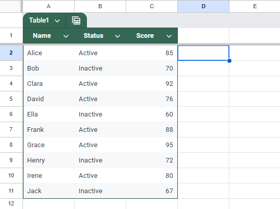
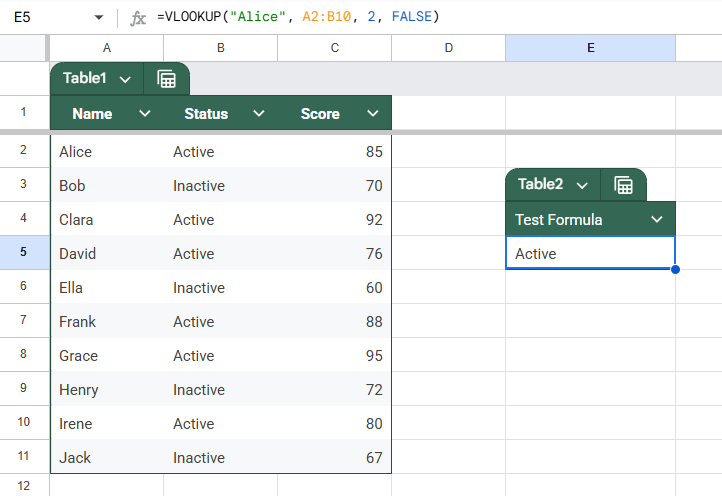
This is the dataset we will be using to demonstrate the methods:
Steps:
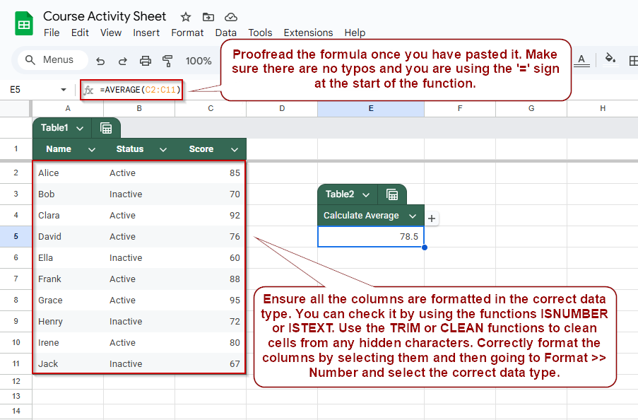
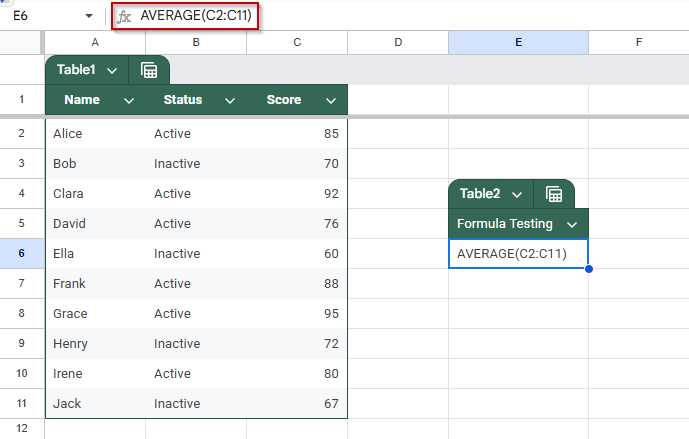
➤ Make sure the formula starts with the equal sign (=). Google Sheets only interprets a formula if it begins with =. Without it, the formula will appear as normal text.
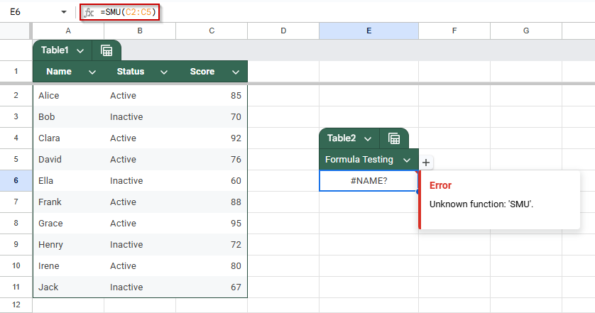
➤ Carefully check the function name for spelling errors. For example, =SUM(C2:C5) is correct, but =SMU(C2:C5) will return a #NAME? error because SMU is not a recognized function.
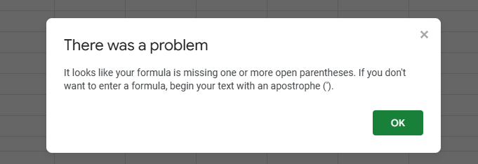
➤ Look over your formula for missing commas, extra parentheses, or incorrect syntax. Even a small mistake in punctuation can cause the formula to break.
➤ Use the formula help tooltip that appears as you type. It can guide you on proper structure and argument order for most built-in functions.
Correct example: =AVERAGE(C2:C11)
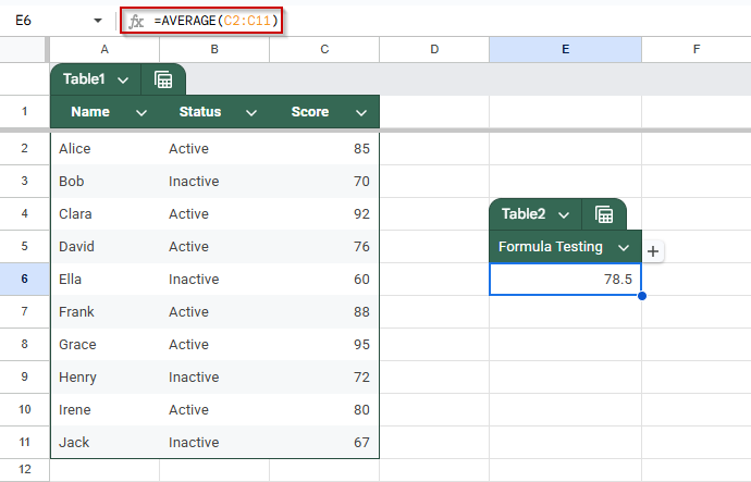
Incorrect example: AVERAGE(C2:C11) (missing the = at the beginning)
Ensure Data Types Match Within Your Formula
Formulas in Google Sheets may not work properly if you are comparing different data types, such as numbers and text. Google Sheets distinguishes between values like 85 (a number) and “85” (a text string), and a mismatch can lead to unexpected results or no result at all. This method helps you identify and resolve these inconsistencies.
Steps:
➤ Use the ISTEXT(cell) and ISNUMBER(cell) functions to check whether a cell contains text or a number. This helps confirm whether your formula is comparing like-for-like data types.

➤ Avoid comparing text strings that look like numbers to actual numeric values. For example, “85” is not equal to 85, even though they look identical in the cell.

➤ If you find that a numeric-looking value is actually stored as text, convert it back to a number by removing any characters that could be causing it to be formatted as a text.
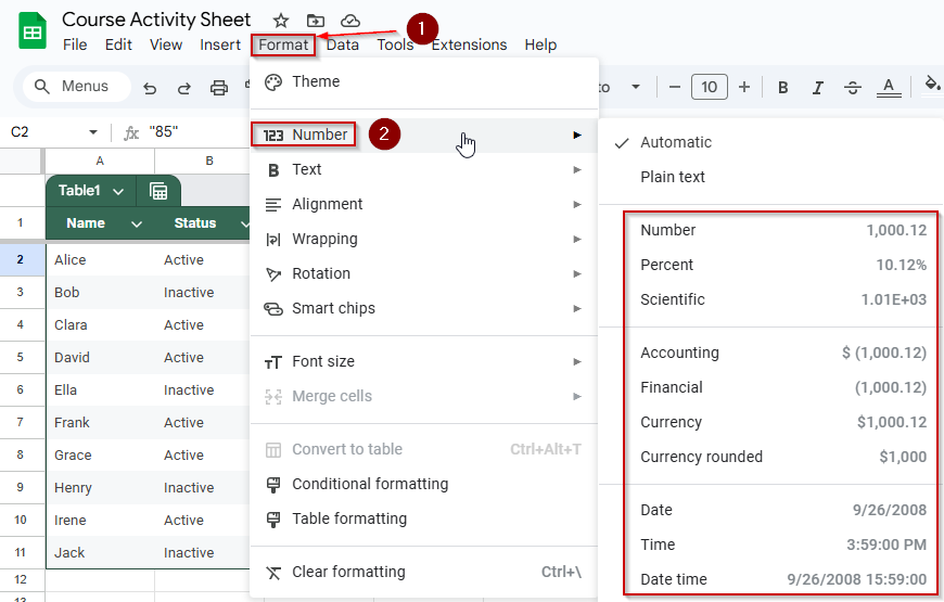
➤ Ensure that any columns used for calculations or comparisons are formatted consistently as either numbers or text, depending on the logic you need. Select your column and then click on Format >> Number. Choose your desired data type for the column from the expanded menu.
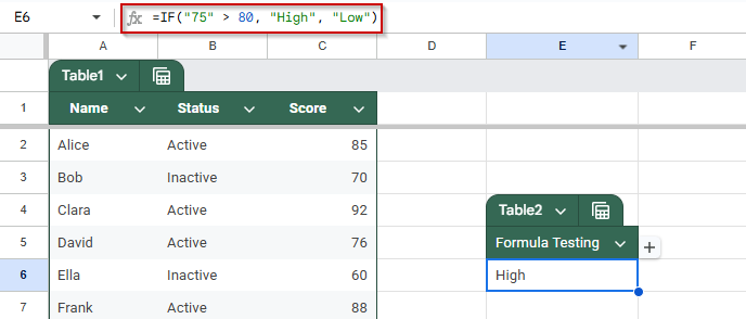
Correct example: =IF(C2 > 80, “High”, “Low”) (works correctly if C2 contains a number)
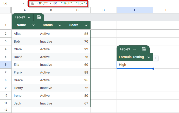
Incorrect example: =IF(“75” > 80, “High”, “Low”) (will not work as expected if “75” is stored as text)
Use TRIM or CLEAN to Remove Hidden Characters
Formulas in Google Sheets can fail when cells contain hidden characters such as extra spaces or non-printable symbols. These characters are not always visible, but they can prevent functions like FILTER, VLOOKUP, or MATCH from returning correct results. This method shows how to clean your data using built-in functions before applying formulas.
Steps:
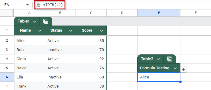
➤ Use the TRIM function to remove unnecessary spaces from text, especially leading or trailing spaces that can interfere with comparisons. For example, =TRIM(A2) will clean up cell A2.
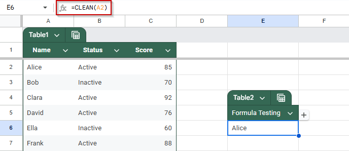
➤ Apply the CLEAN function to strip non-printable or special characters that may have been copied in from other sources like PDFs or exported files. Example: =CLEAN(A2).
➤ To prepare your entire dataset, create a new column where you apply TRIM or CLEAN across your data range. This ensures all values used in formulas are uniform and clean.
➤ Once cleaned, you can confidently run formulas like FILTER, VLOOKUP, or COUNTIF that depend on consistent and exact matches between values.
Correct example: =FILTER(A2:C11, TRIM(B2:B11)=”Active”).
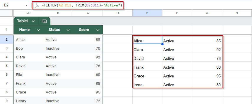
This ensures the comparison to “Active” works even if extra spaces are present in column B.
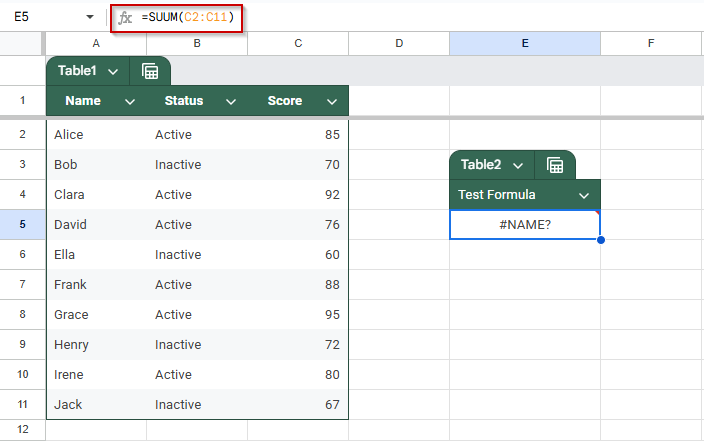
Resolve the #NAME? Error by Checking Formula Names and Strings
The #NAME? error occurs when Google Sheets doesn’t recognize something you’ve typed in a formula. This often happens due to misspelled function names, missing quotation marks around text, undefined named ranges, or using functions that are exclusive to Excel. Identifying and correcting these small input mistakes will usually resolve the error quickly.
Steps:
➤ Double-check the function name for typos. For instance, use =SUM(C2:C11) instead of =SUUM(C2:C11).
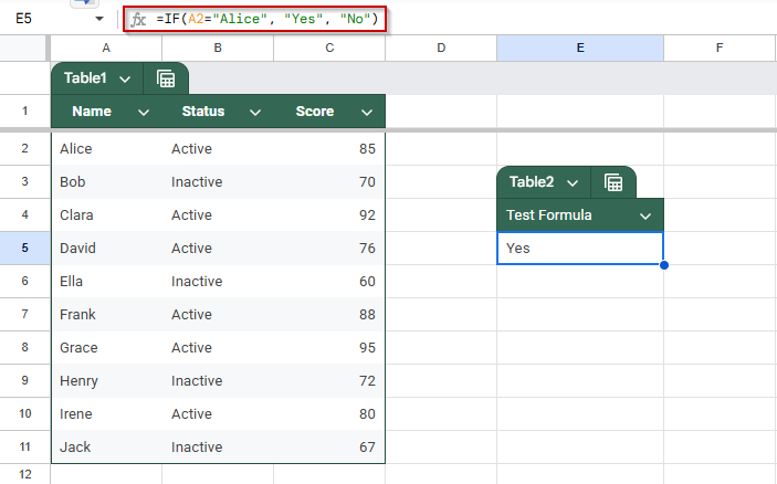
➤ Ensure that any text values in your formula are enclosed in double quotation marks. For example, use “Apples”, not just Apples.
If you want to check if cell A1 contains the word Apples, the correct formula is:
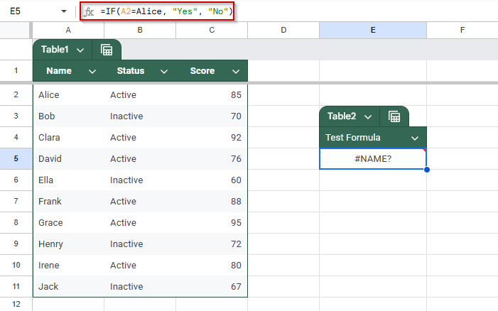
=IF(A2=”Alice”, “Yes”, “No”)
Incorrect version that causes #NAME? error: =IF(A2=Alice, “Yes”, “No”) (missing quotes around Apples)
➤ If using named ranges, make sure the name exists and is spelled exactly as defined.
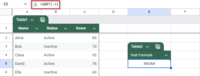
Fixing Mathematical Input Errors That Cause #NUM! in Google Sheets
The #NUM! error occurs when a formula tries to perform an invalid or undefined mathematical operation. This can include impossible calculations like the square root of a negative number, exponential overflows, or functions requiring specific input ranges. Understanding where the numeric logic fails helps you correct the formula and avoid this common mistake.
Steps:
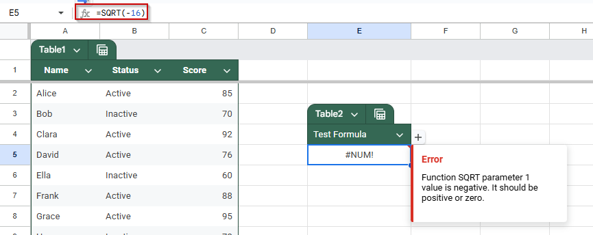
➤ Avoid invalid calculations like taking the square root of a negative number. For example, =SQRT(-4) will return a #NUM! Error.
➤ Check that input values fall within the expected range for specific financial or iterative functions such as =IRR or =RATE.
- Correct example: =IRR({-1000, 500, 400, 300})
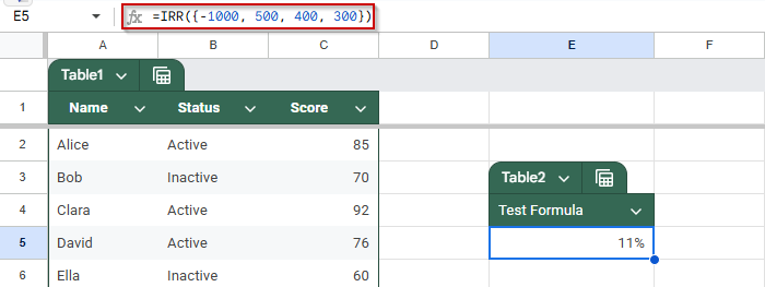
This returns a valid percentage, since the cash inflow exceeds the investment over time.
- Incorrect example: =IRR({-1000, -100, -50})
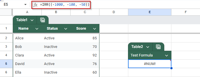
This returns #NUM! because the cash flows never exceed the initial investment, and IRR fails to converge.
➤ Make sure numbers are within Google Sheets’ supported limits. Extremely large or small values may cause overflow or rounding errors.
➤ Review formulas for recursive logic or circular references that could generate infinite or excessive iterations.
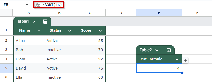
- Correct example: =SQRT(16)
- Incorrect example: =SQRT(-16) (negative number inside SQRT triggers #NUM!)
Prevent Division by Zero Errors with Defensive Formula Logic
The #DIV/0! error occurs when a formula attempts to divide a number by zero or by a blank cell. While mathematically undefined, this error is easy to prevent by building logic into your formulas to check for empty or zero values before dividing. Adding basic checks helps keep your sheet error-free and user-friendly.
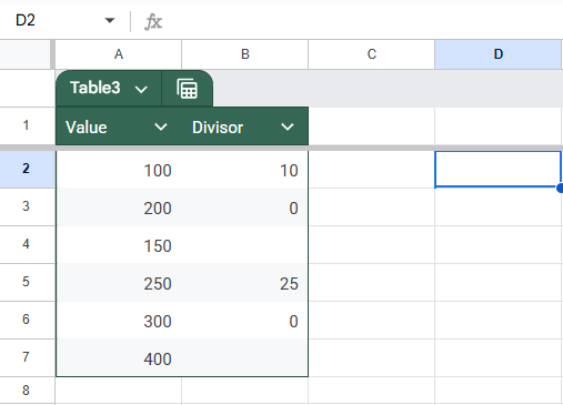
This is the dataset we will be using to demonstrate this method:
Steps:
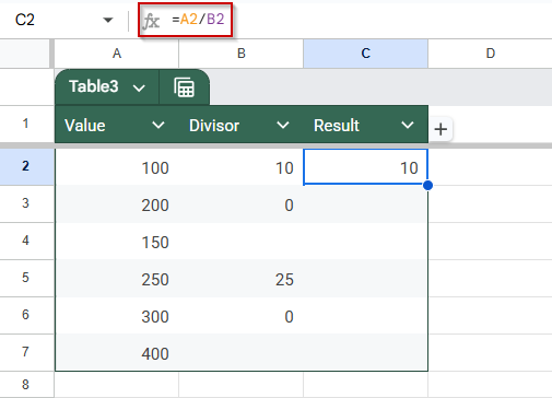
➤ Check that the denominator in your formula is not zero or empty. For instance, in =A2/B2, confirm that cell B2 contains a nonzero number.
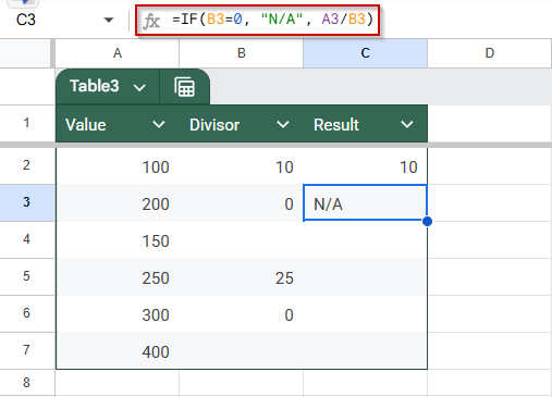
➤ Use conditional logic functions like IF to display a custom result (e.g., “N/A”) when the divisor is zero.
➤ If needed, replace empty cells with default values to avoid triggering the error unexpectedly.
- Correct example: =IF(B3=0, “N/A”, A3/B3)
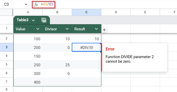
- Incorrect example: =A3/B3 (returns #DIV/0! if B1 is zero or blank)
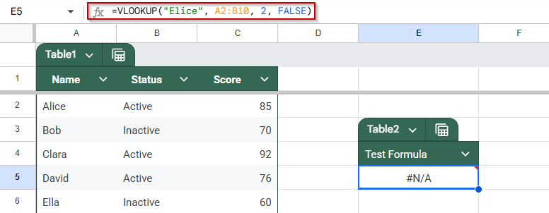
Handle Missing Lookup Matches That Trigger #N/A Errors
The #N/A error in Google Sheets signals that a formula couldn’t find the value it was looking for. This usually happens with functions like VLOOKUP, MATCH, or XLOOKUP when the lookup value doesn’t exist in the specified range or when the range is misconfigured. Instead of allowing this error to appear, you can build in logic to manage it gracefully.
Steps:
➤ Verify that the lookup value exists in the specified range. A small typo or mismatch will prevent a match and cause #N/A.
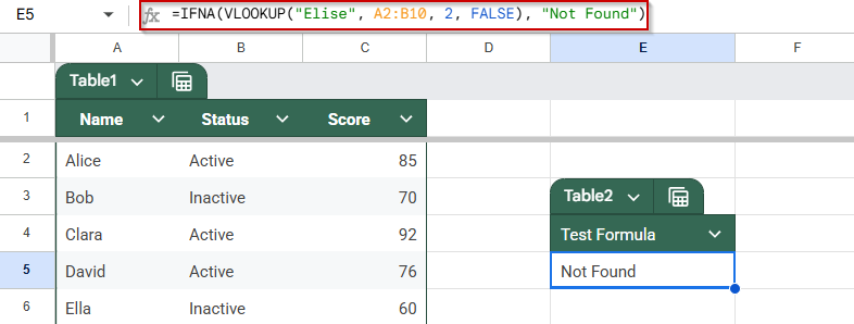
➤ Use IFNA or IFERROR functions to handle the error and display a more user-friendly message like “Not Found”.
➤ Make sure the column index (for VLOOKUP or XLOOKUP) is valid and falls within the range of the lookup table.
- Correct example: =IFNA(VLOOKUP(“Elise”, A2:B10, 2, FALSE), “Not Found”)
- Incorrect example: =VLOOKUP(“Alice”, A2:B15, 3, FALSE) (column index out of range returns #N/A)
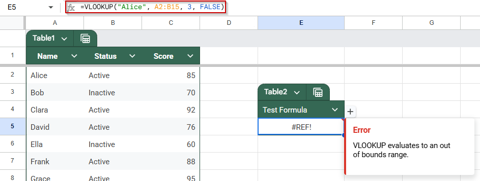
Fix Broken Cell References That Cause #REF! Errors
The #REF! error in Google Sheets appears when a formula points to an invalid or deleted cell reference. This typically occurs after deleting rows or columns on which the formula depends, or when referencing a cell outside the allowable range. Restoring or correcting the reference is key to fixing the issue.
Steps:
➤ Avoid deleting rows or columns that are referenced in existing formulas. Deletion will break the reference and return #REF!.
Before Deleting:
After Deleting:
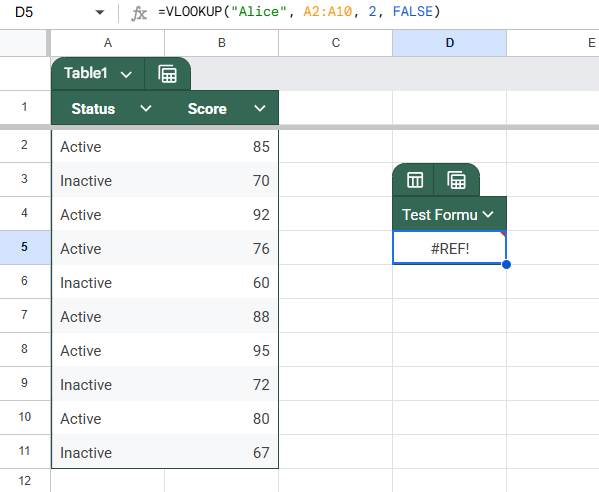
➤ When you see #REF! in a formula, click the cell to inspect the formula bar. Re-enter or manually fix the broken reference.
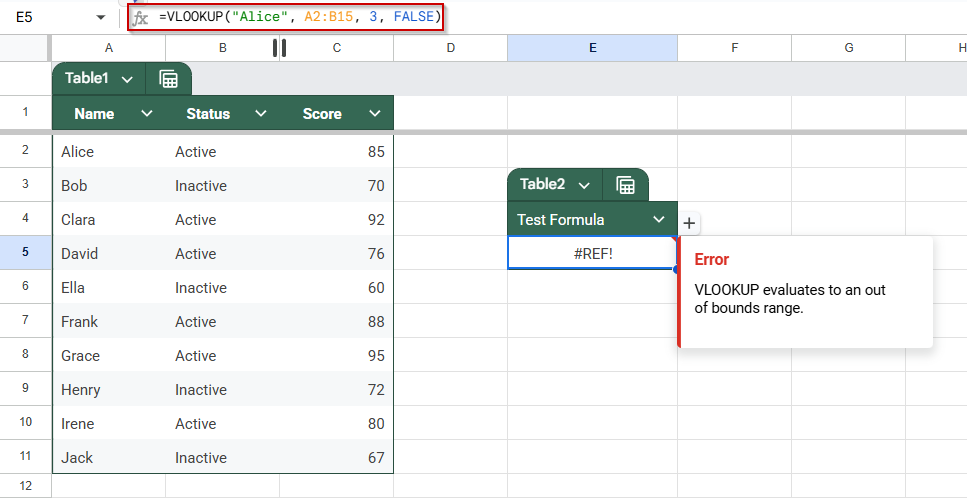
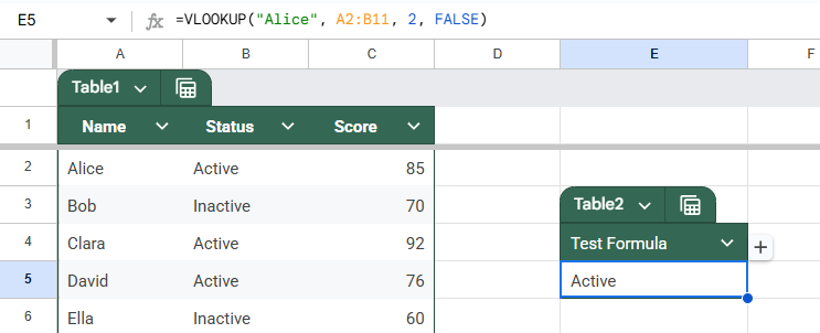
In this case, you need to select a range that is within the bounds of the 3rd column index you have specified in the formula. To fix thi,s you can either change the column index to 2 or increase the bounds of your range.
➤ Be cautious when using INDIRECT or named ranges. These do not auto-update if source cells are deleted or changed.
Resolve Incompatible Data Types That Cause #VALUE! Errors
The #VALUE! error occurs when a formula receives an unexpected data type, such as trying to perform math on text, combining incompatible values, or referencing improperly formatted cells. This error signals that something in the formula cannot be processed as expected, and usually requires a closer look at the inputs involved.
Steps:
➤ Make sure all values in a calculation are numeric. For example, =”Apple” + 5 will return #VALUE! because text can’t be added to a number.
➤ Use ISNUMBER and ISTEXT to verify the data types of each input cell.
➤ Apply the VALUE function to convert text strings that look like numbers (e.g., “85”) into actual numeric values.
➤ Use TRIM or CLEAN to remove hidden characters that may be affecting cell content.
➤ Be cautious with array formulas or custom functions—these may return #VALUE! if part of the input range includes invalid data types.
Correct example: =A1 + 5 (works if A1 contains a number)
Incorrect example: =”Test” + 5 (mixing text and numbers triggers #VALUE!)
Frequently Asked Questions
Why is my Google Sheets formula returning a blank result?
This usually happens when the formula is referencing empty or non-matching data. Double-check your criteria and ranges to ensure they contain values.
Why do I see a formula as plain text instead of a result?
Your formula might be entered without =, or the cell is formatted as Plain Text. Change the cell format to Automatic and re-enter the formula with =.
Can formatting affect my formula?
Yes. If a number is stored as text or if a cell has hidden spaces, it may break logic-based formulas. Use VALUE, TRIM, or CLEAN to sanitize data.
Why am I getting a #NAME? Error?
That error usually means there’s a typo in the formula name, or you’re using a function that doesn’t exist in Google Sheets (e.g., Excel-only functions).
Wrapping Up
If your formula isn’t working in Google Sheets, don’t panic. Most issues come down to minor problems like typos, incorrect cell references, hidden spaces, or mismatched data types. By going through these common troubleshooting steps, you can quickly identify and fix the issue, and get your formulas working exactly as expected. For the best results, always clean your data, double-check syntax, and use functions native to Google Sheets.