What-if analysis helps you test different assumptions or inputs in a spreadsheet to see how they affect the final outcome. Whether you’re planning a budget, tracking inventory, or forecasting sales, Google Sheets offers flexible tools to run scenario-based calculations with ease.
In this article, we’ll show you methods on how to perform what-if analysis using basic formulas, data tables, and goal seek techniques, all within Google Sheets.
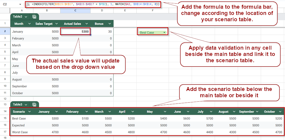
Steps to simulate Scenario Manager for What-If Analysis in Google Sheets:
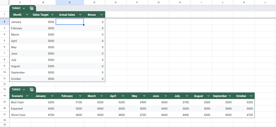
➤ Create a “Scenarios” table with different cases like Best Case, Expected, and Worst Case, each with values for Actual Sales.
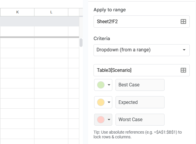
➤ Add a drop-down menu using Data >> Data validation. Choose the Drop-down and enter the scenario names (Best Case, Expected, Worst Case). Place it in a cell like F2.
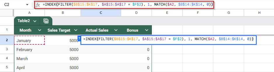
➤ Use this formula in your Actual Sales cell (e.g., C2 for Jan) to link it with the scenario selected in the drop-down:
=INDEX(FILTER($B$15:$D$17, $A$15:$A$17 = $F$2), 1, MATCH($A2, $B$14:$D$14, 0))
➤ Make sure $B$15:$D$17 covers your scenario data, $A$15:$A$17 holds scenario names, $F$2 is your drop-down cell, and $A2 is the month (e.g., Jan, Feb).
➤ Use this formula for bonus calculation in a new column: =IF(C2 > B2, 200, 0)
What Is What-If Analysis in Google Sheets?
What-if analysis in Google Sheets is a decision-support technique that allows you to test different scenarios by modifying input values and observing the impact on the outcome. It helps users explore the potential impact of variables on a specific result without altering the original data permanently.
| Uses of What-If Analysis |
|---|
| ➠ Predict financial outcomes (like profit or commission) based on sales numbers |
| ➠ Adjust pricing models to see how revenue changes |
| ➠ Test best-case, worst-case, and expected scenarios |
| ➠ Reverse-engineer inputs using formulas or add-ons such as Goal Seek for Google Sheets. |
In Google Sheets, what-if analysis is typically performed using formulas such as IF, VLOOKUP, or INDEX, along with tools like drop-down menus and data tables to dynamically visualize the results. It’s highly useful for budgeting, forecasting, and business planning
Use the IF Function to Test Bonus Scenarios
Using the IF function is a straightforward way to perform what-if analysis in Google Sheets. It helps you test specific conditions, like whether a salesperson should receive a bonus for exceeding a sales target, and instantly see the result based on the values entered. This is useful for modeling outcomes that depend on meeting thresholds.
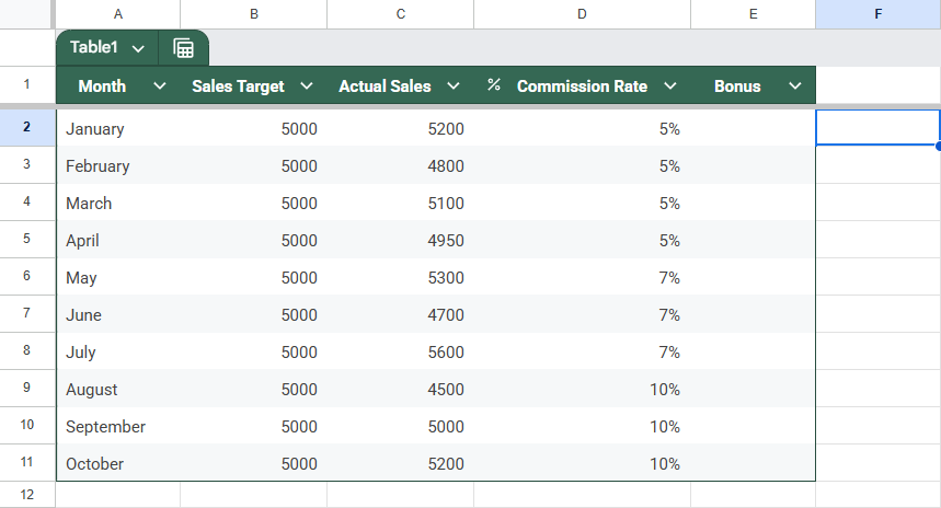
This is the sample dataset that we will be using to demonstrate the methods:
Steps:
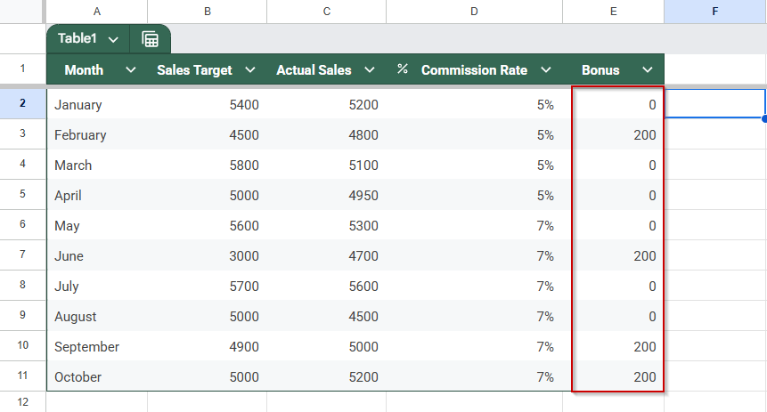
➤ Add the formula =IF(C2 > B2, 200, 0) in the first cell of the Bonus column.
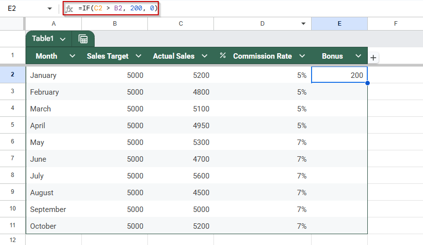
This formula checks if actual sales in cell C2 are greater than the target in B2. If true, it returns 200 (the bonus amount); otherwise, it returns 0.
➤ Drag the fill handle down to apply the formula to all rows in the dataset.
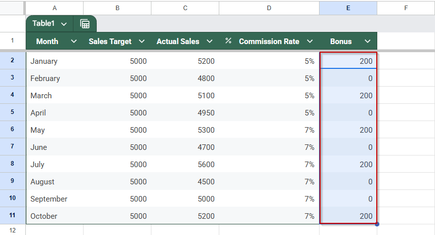
➤ Adjust the Sales Target values in column B or Actual Sales in column C to test different performance scenarios.
➤ Observe how the Bonus column updates instantly based on your inputs.
This method allows you to quickly simulate bonus payouts under various conditions and visualize the impact of altering sales performance. Please note that this method is not applicable to commission rates. We will demonstrate the correct method to calculate the bonus with the commission rate further down this guide.
Utilize Data Columns for Multi-Scenario Testing
Data columns are a great way to perform what-if analysis in Google Sheets by comparing multiple scenarios at once. For instance, if you want to see how different commission rates affect total earnings, you can set up a simple table where each row or column represents a different rate. This lets you test various inputs side-by-side without rewriting your formula each time.
Steps:
➤ Create a column listing different commission rates, such as 5%, 7%, and 10%. We already have in our case.
➤ In a separate cell, input the formula to calculate total commission, such as =C2 * $B$1, where C2 is the actual sales and $B$1 holds the commission rate.
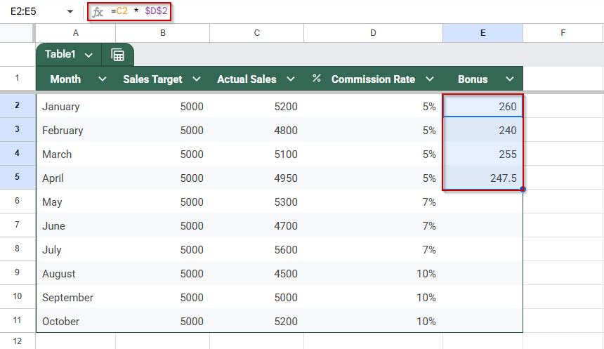
➤ Use absolute cell references (with $) to lock the commission rate when copying the formula.
➤ Drag the formula across rows or columns to apply it to all listed scenarios with the same scenario.
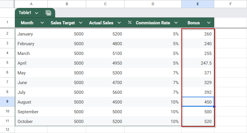
➤ Modify the rate in the reference cell and see how commission values update instantly across the table.

This approach provides a clear view of how varying a single input (such as the rate) affects the outcome, enabling quick decision-making based on multiple possibilities.
Apply Goal Seek to Reverse Engineer
Google Sheets doesn’t have a built-in Goal Seek tool like Excel, but you can still reverse-calculate input values by using manual iterations or third-party add-ons. This technique is useful when you know the desired result and want to figure out the input required to reach it. For example, if you want to find out how much you need to sell to earn a $300 commission at a 5% rate, you can work backwards using a simple formula.
Manual Goal Seek
Steps:
➤ In one cell, enter your formula to calculate commission, such as =C2 * 5%, where C2 is the sales value you’re adjusting.
Using Add-on
Steps:
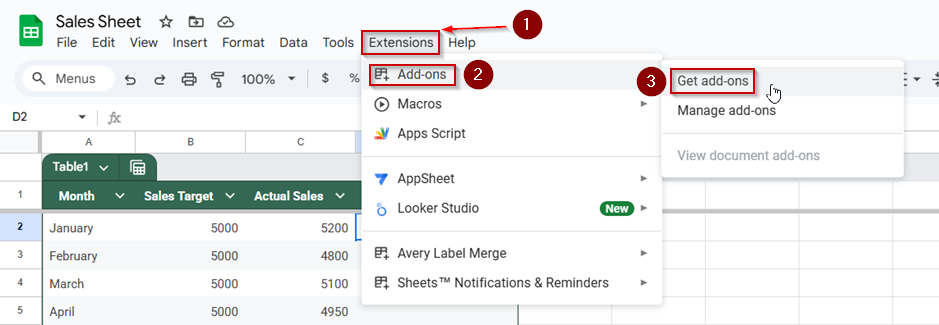
➤ Go to Extensions >> Add-ons >> Get add-ons and search for “Goal Seek.”
➤ Install a Goal Seek add-on like “Goal Seek for Sheets”.

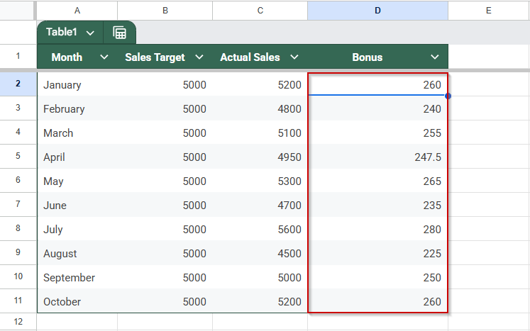
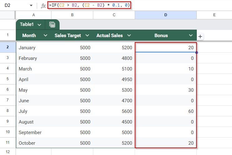
➤ In your dataset, first enter the following formula in cell D2 to calculate the bonus:
=IF(C2 > B2, (C2 – B2) * 0.1, 0)
➤ Drag the formula down to fill the Bonus column for all months (D2 to D11)
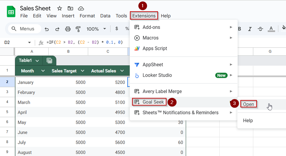
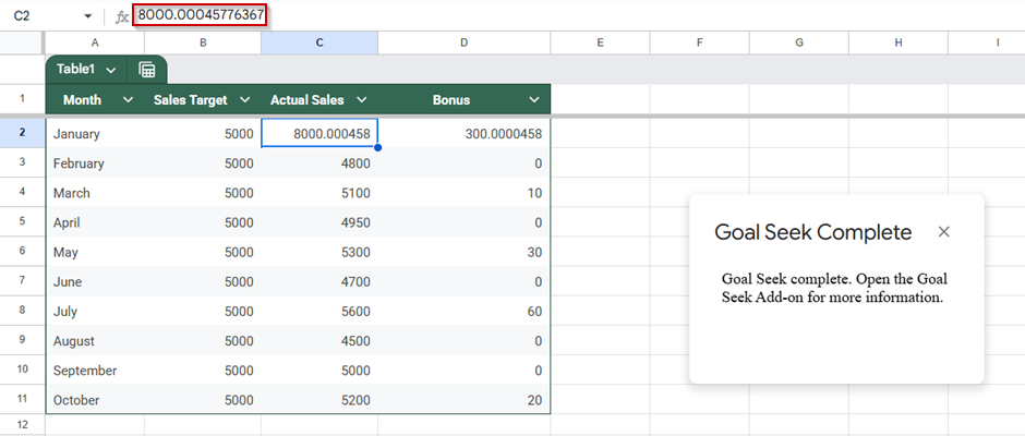
➤ Go to Extensions >> Goal Seek for Sheets >> Open.
➤ In the Goal Seek sidebar:
- Set Cell to D2 (this is the bonus formula cell for January)
- To Value to enter your target bonus (e.g., 300)
- By Changing Cell to C2 (this is the Actual Sales cell for January)
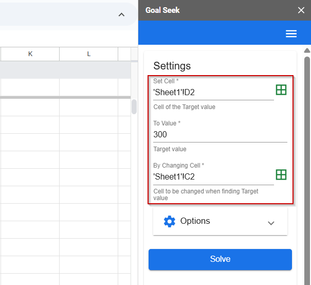
➤ Click Solve. Goal Seek will adjust the Actual Sales value to achieve the desired bonus.
➤ Repeat the process for other months by updating the Set Cell and Input Cell accordingly (e.g., D3/C3 for February, D4/C4 for March, etc.).
Using Scenario Manager (Simulated in Google Sheets)
This method allows you to simulate Excel’s Scenario Manager using drop-down menus and formulas in Google Sheets. It’s especially useful for comparing multiple business scenarios (like Best Case, Worst Case, and Expected) by automatically updating your dataset based on the selected scenario.
Steps:
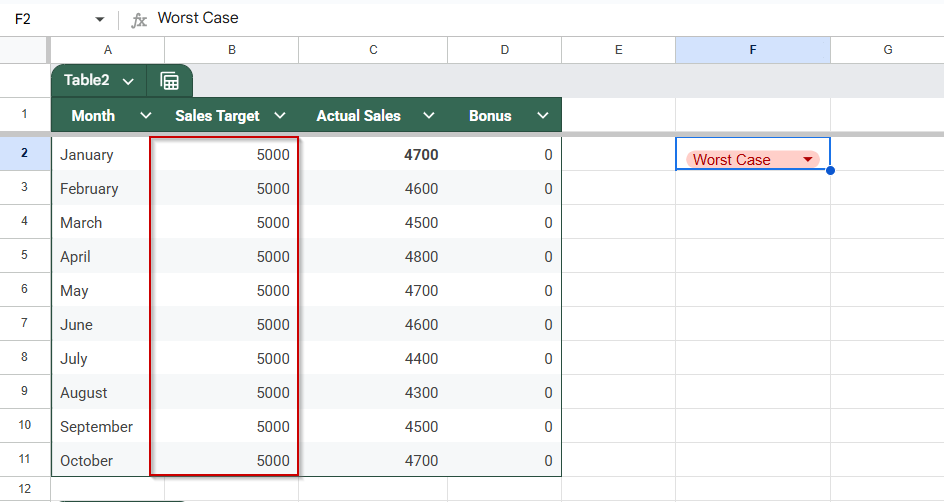
➤ Create a section (e.g., to the right or below your table) labeled “Scenarios”. Add multiple rows with different scenario values for Actual Sales (e.g., Best Case, Worst Case, Expected).
➤ Next to each scenario label, enter the corresponding Actual Sales values in the same format as your table. For example:
➤ Go to Data >> Data validation and choose Drop-down (from a range). Create a drop-down list with the scenario names (e.g., Best Case, Expected, Worst Case). Place the drop-down in a new cell, say F2.
➤ In your original table under the Actual Sales column, use a VLOOKUP or INDEX-MATCH formula that pulls the actual sales based on the selected scenario. Example for January (C2):
=INDEX(FILTER($B$15:$K$17, $A$15:$A$17 = $F$2), 1, MATCH($A2, $B$14:$K$14, 0))
Adjust the ranges based on where you placed your scenario table and drop-down)
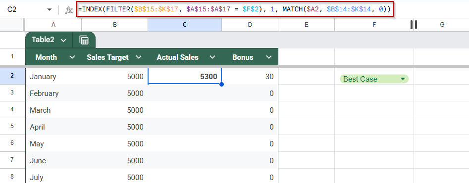
➤ The Actual Sales values will now dynamically update based on the selected scenario, and your Bonus column formulas will update automatically as well.
Frequently Asked Questions
Does Google Sheets have a built-in Goal Seek feature?
No, Google Sheets does not have a native Goal Seek feature like Excel. However, you can simulate it manually or install a Goal Seek add-on.
Can I run multiple scenarios in Google Sheets?
Yes, by setting up data tables with different input values, you can easily compare multiple scenarios and see how outcomes like revenue or profit change.
What is the best way to perform a basic what-if analysis?
Using IF formulas is the simplest way. You can test how changing input values, like sales targets or commissions, affects results by adjusting those cells.
Is the What-If Analysis feature available in the mobile app?
No, advanced what-if tools like Goal Seek or data tables work best on a desktop. The mobile app is limited to complex analysis and formula testing.
Wrapping Up
What-if analysis in Google Sheets is a powerful tool for testing assumptions, projecting future results, and making smarter decisions. Whether you use simple IF logic, build dynamic data tables, or simulate reverse outcomes with Goal Seek, these techniques will help you adapt to real-world scenarios with confidence.
By practicing these methods on small datasets, you’ll gain the flexibility to analyze anything from business forecasts to personal budgets, all within Google Sheets.