Google Sheets makes it easy to sum values based on specific conditions using the SUMIF function. However, when you need to evaluate more than one condition, such as summing sales only for a certain product and region, you’ll need to use SUMIFS instead.
In this article, you’ll learn how to use both SUMIF and SUMIFS in Google Sheets, explore real-world examples, and work with sample datasets that help you apply what you learn immediately.
Steps to use SUMIFS in Google Sheets for summing with multiple criteria:
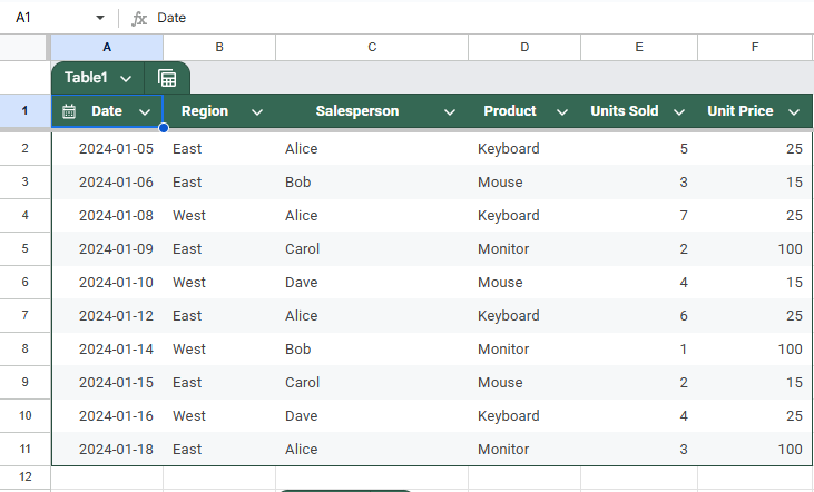
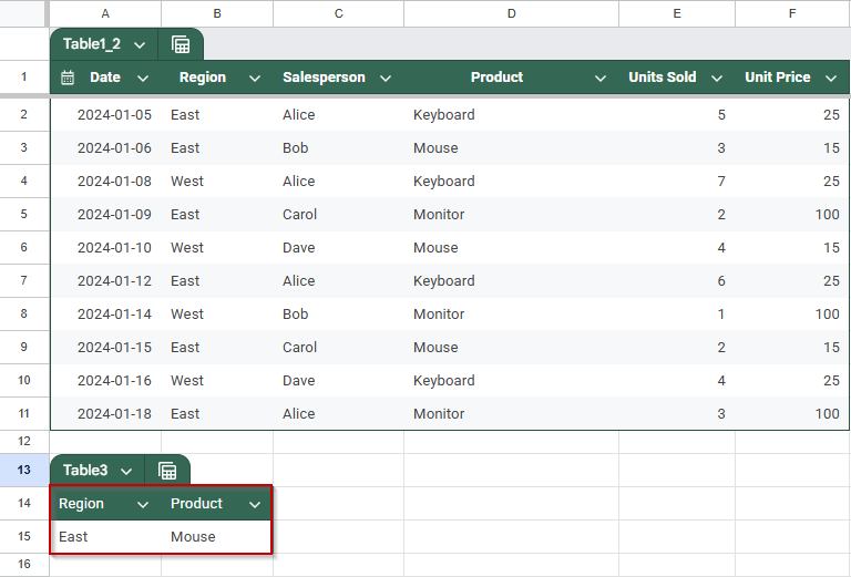
➤ Use the sample dataset in range A1:F11, which includes Region, Product, and Units Sold.
➤ Select a blank cell (e.g., H2) to display your result.
➤ Enter the formula:
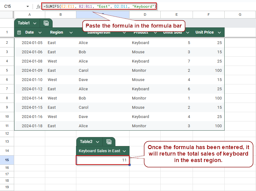
=SUMIFS(E2:E11, B2:B11, “East”, D2:D11, “Keyboard”)
➤ E2:E11: Range to sum (Units Sold).
➤ B2:B11, “East”: First condition, Region must be East.
➤ D2:D11, “Keyboard”: Second condition, Product must be Keyboard.
➤ Press Enter to get the total (in this example, 11 units).
Why Use SUMIFS Instead of SUMIF for Multiple Criteria in Google Sheets?
The SUMIF function is limited to evaluating a single condition, which makes it unsuitable for scenarios that require filtering by multiple criteria, such as summing values where both the product is “Apples” and the delivery status is “Delivered.”
In such cases, the SUMIFS function is a better choice. It allows you to apply multiple conditions across different columns, making your analysis more accurate and flexible. By specifying a sum range followed by pairs of criteria ranges and their respective conditions, SUMIFS ensures that only rows that meet all the criteria are included in the total. This makes it ideal for detailed reporting and data filtering tasks in Google Sheets.
Use SUMIFS to Sum with Multiple Criteria
This method demonstrates how to use the SUMIFS function in Google Sheets to sum values based on multiple conditions. It’s perfect for scenarios where you want to narrow down results, like totaling only “Keyboard” sales in the “East” region from a full sales dataset. This approach is ideal for filtered analysis in sales reporting, forecasting, and dashboards.
We’ll use this dataset (assumed to be in range A1:F11):
Steps:
➤ Select a blank cell where you want the result to appear (e.g., C15).
➤ Enter the following formula:
=SUMIFS(E2:E11, B2:B11, “East”, D2:D11, “Keyboard”)
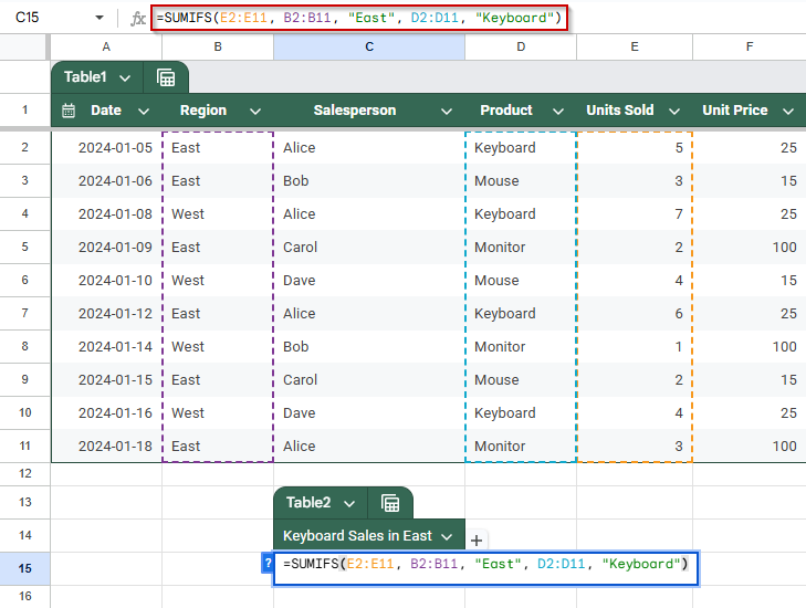
➧ B2:B11, East: Applies the first condition: Region must be East.
➧ D2:D11, Keyboard: Applies the second condition: Product must be Keyboard.
➤ Press Enter
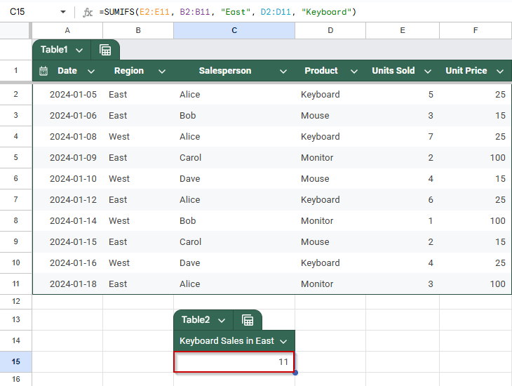
Once entered, the formula will return the total number of units sold for Keyboards in the East region (in this case, 5 + 6 = 11).
Make SUMIFS Interactive Using Cell References
This method demonstrates how to use cell references instead of hardcoded values in your SUMIFS formula. This makes your analysis interactive, just change the cell values to instantly update results. It’s perfect for dynamic dashboards where users want to control filters like Region or Product.
Steps:
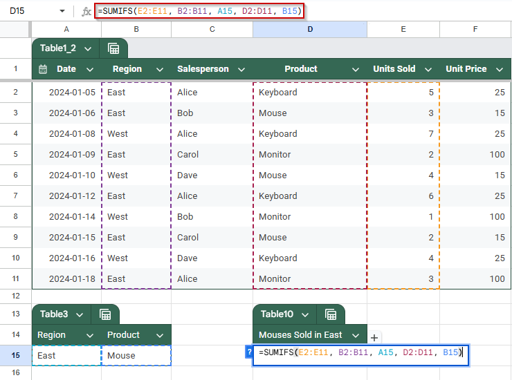
➤ Set up your criteria cells. In A14, enter Region. In A15, enter the region you want to filter by (e.g., East). In B14, enter Product. B15, enter the product to filter by (e.g., Mouse)
➤ Select a blank cell where you want the total result to appear (e.g., J2)
➤ Enter the following formula:
=SUMIFS(E2:E11, B2:B11, H2, D2:D11, I2)
➤ Press Enter
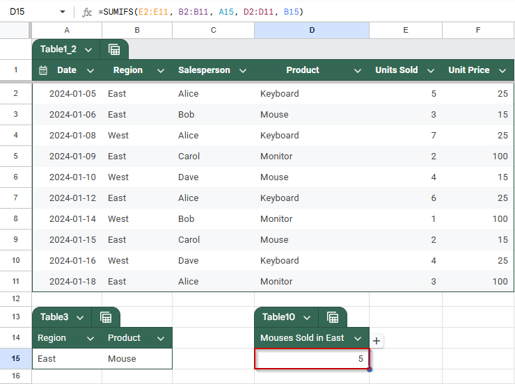
Any time you change the values in H2 or I2, the result updates automatically. This makes your sheet clean, flexible, and easy to use.
Summing Data with Multiple Criteria Using SUMIFS
This method shows how to sum values in Google Sheets when more than one condition must be true at the same time, also called AND logic. Instead of using complex array formulas like SUMPRODUCT, you’ll use SUMIFS, a simpler and more readable function. This is useful for analyzing sales or inventory where you want to total only specific combinations, such as sales of a particular product that have been delivered.
Steps:
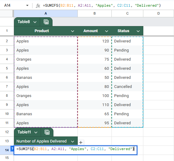
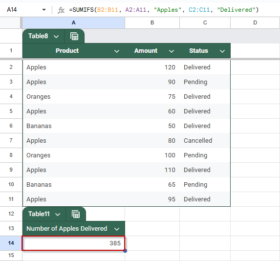
➤ Select a blank cell where you want the result to appear (e.g., A14)
➤ Enter the following formula:
=SUMIFS(B2:B11, A2:A11, “Apples”, C2:C11, “Delivered”)
➤ Press Enter
➤ To make the formula dynamic using cell inputs, enter the keywords “Apple” in C13, and “Delivered” in C14.
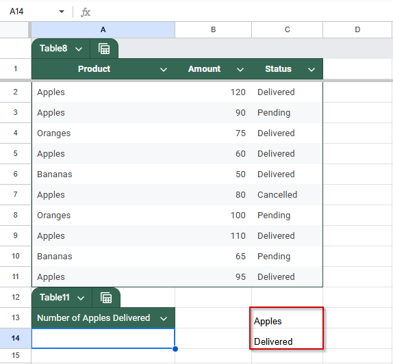
➤ Use this formula:
=SUMIFS(B2:B11, A2:A11, C13, C2:C11, C14)
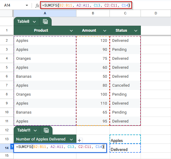
➧ A2:A11, Apples: First condition, Product must be Apples
➧ C2:C11, Delivered: Second condition, Status must be Delivered
➧ C13 and C14 (optional): Use these cells for user-entered criteria (e.g., C13 = Apples, C14 = Delivered)
➤ Press Enter
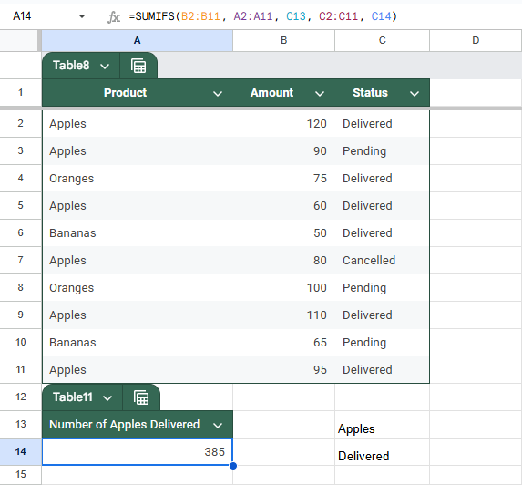
The formula will return the total of all rows that meet both criteria, product and delivery status.
Utilizing Wildcard Characters for Partial Matches using SUMIFS
This method shows how to sum values based on partial text matches using wildcard characters in your criteria. It’s useful when you don’t remember the exact text but know part of it, like a product name containing “Blox.”
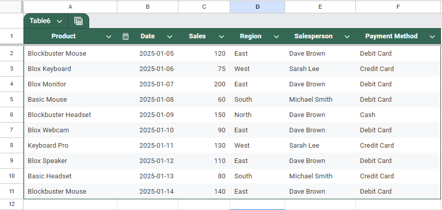
This is a sample dataset we will be using to demonstrate this method.
Steps:
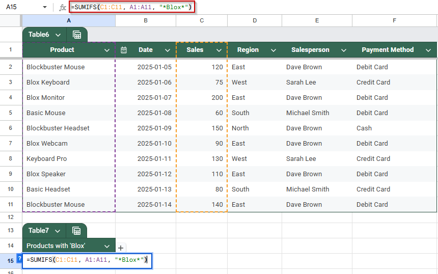
➤ In a blank cell, enter the following formula to sum sales where the product name contains “Blox”:
=SUMIFS(C1:C11, A1:A11, “*Blox*”)
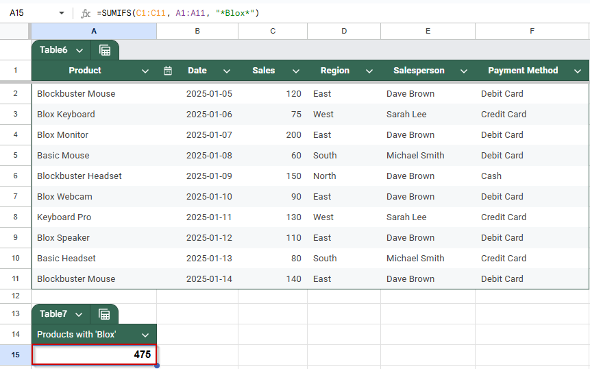
➤ Press Enter
➤ To apply multiple criteria with partial text matching, use:
=SUMIFS(C1:C11, A1:A11, “*Blox*”, E1:E11, “Dave Brown”, F1:F11, “Debit Card”)
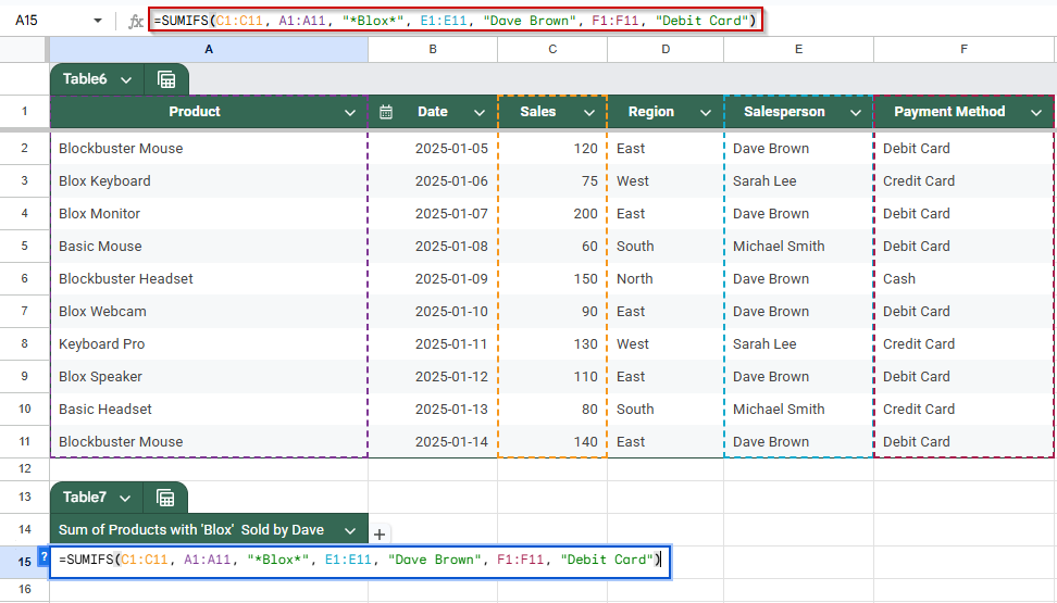
➧ A1:A11, Blox: Product name contains Blox (partial match using wildcards)
➧ E1:E11, Dave Brown: Additional criterion (e.g., salesperson)
➧ F1:F11, Debit Card: Another condition (e.g., payment method)
➤ Press Enter
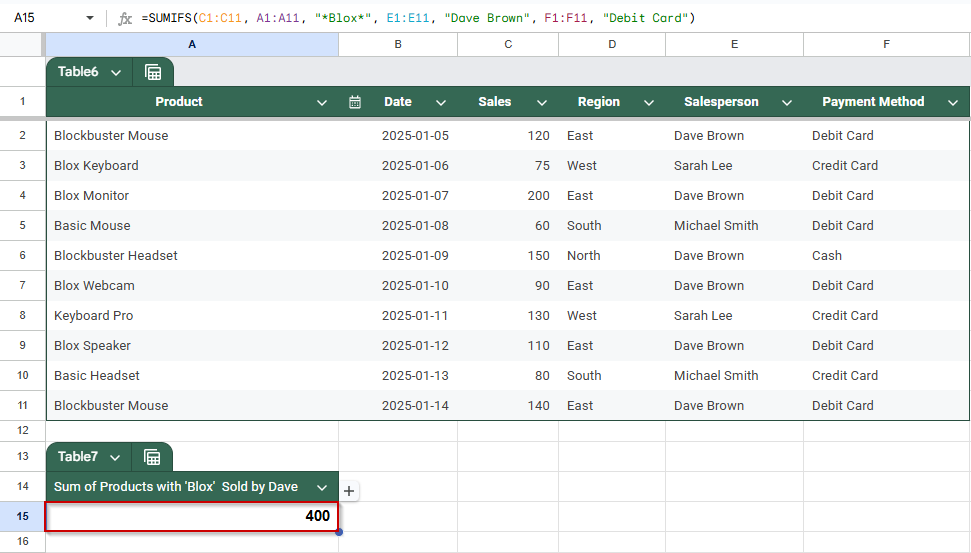
Now, the formula sums all values that meet the multiple conditions, including partial matches on the product name.
Alternative Method: Handle OR Conditions Using SUMPRODUCT in Google Sheets
This method explains how to sum values when you need to apply OR logic across multiple criteria, a task that SUMIFS cannot perform directly. For instance, if you want to find total Units Sold for the product “Mouse” across both the East and West regions, SUMPRODUCT is the best tool to use.
We’ll use the same dataset from earlier (A1:F11), which includes sales records by region, product, and units sold.
Steps:
➤ Identify the criteria ranges. Region is in column B (B2:B11). Product is in column D (D2:D11). Units Sold is in column E (E2:E11).
➤ Build the first part of the formula to handle Region = “East” AND Product = “Mouse”:
=SUMPRODUCT((B2:B11=”East”)*(D2:D11=”Mouse”)*E2:E11)
➤ Build the second part of the formula for Region = “West” AND Product = “Mouse”:
=SUMPRODUCT((B2:B11=”West”)*(D2:D11=”Mouse”)*E2:E11)
➤ Combine both parts with a + to apply the OR condition and paste it on any cell:
=SUMPRODUCT((B2:B11=”East”)*(D2:D11=”Mouse”)*E2:E11) + SUMPRODUCT((B2:B11=”West”)*(D2:D11=”Mouse”)*E2:E11)
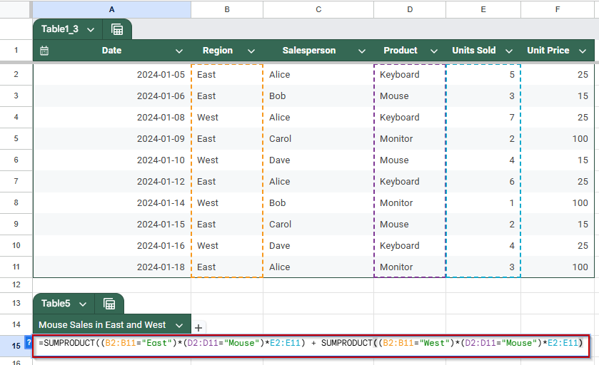
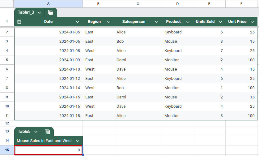
➤ Press Enter to return the total Units Sold where the Region is East or West and Product is Mouse.
Frequently Asked Questions
How do I use SUMIFS with multiple conditions in Google Sheets?
Use =SUMIFS(sum_range, criteria_range1, criteria1, …) to sum values based on multiple criteria. Each condition must match its range and be written in pairs.
Can SUMIF handle more than one criterion?
No, SUMIF supports only one condition. Use SUMIFS instead for multiple criteria, or SUMPRODUCT when using OR logic or more advanced matching.
How do I make SUMIFS dynamic using cell references?
Replace hard coded criteria with cell references, like =SUMIFS(E2:E11, B2:B11, H2, D2:D11, I2), so the formula updates automatically when input values change.
What if I need to use OR logic in my sum conditions?
Use SUMPRODUCT to apply OR logic, combining multiple conditional sums. For example, sum where Region is East or West, and Product is Mouse.
Wrapping Up
Mastering SUMIF and SUMIFS in Google Sheets allows you to efficiently analyze data based on specific conditions, whether it’s summing sales by product, filtering by region, or handling multiple criteria. For even more flexibility, using cell references makes your formulas dynamic, while SUMPRODUCT handles advanced logic like OR conditions that SUMIFS doesn’t support. With these tools, you can turn raw data into actionable insights without ever touching a pivot table or writing complex scripts.