
When working with multiple datasets, Google Sheets users often need to automatically move data between tabs. Users look for this solution when they want to create a master sheet that combines data from multiple source sheets or when they need a way to display real-time changes without having to make any changes themselves. This is helpful for project dashboards, multi-departmental reports, attendance tracking, and workbooks for team collaboration.
To automatically copy data from one Google Sheets sheet to another, do the following:
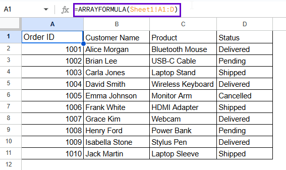
➤ Go to the target sheet, which is Sheet2.
➤ In the destination cell, type:
=ARRAYFORMULA(Sheet1!A2:D)
➤ Press Enter to apply the formula. The whole column will be copied, and it will change automatically when you add new data.
This article will show you different ways to automatically copy data from one sheet to another in Google Sheets. We’ll go over basic formulas, ARRAYFORMULA, and even more complex methods that use IMPORTRANGE, FILTER, QUERY, and Apps Script. You’ll also find answers to frequently asked questions and tips for resolving problems to make sure the automation works perfectly for you.
Using Direct Cell Reference to Copy Data from One Sheet to Another
This procedure is the most straightforward way to copy data from one Google Sheets sheet to another. You can copy a certain range of cells from a source sheet to a destination sheet by using a direct cell reference.
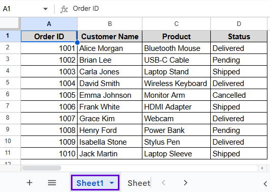
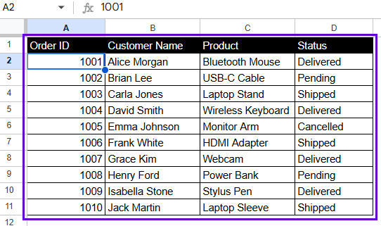
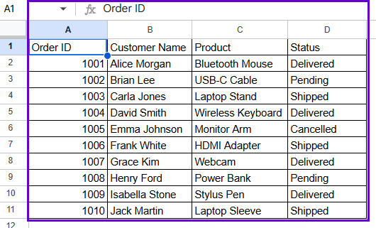
Here, the dataset lists the order information for an online store with details like Order ID, Customer Name, Product, and Status in Sheet1.
Now, we want to automatically show the product data from Sheet1 in the other sheets in the following dataset. When you want to copy a set range of data, the easiest way is to use direct cell references.
Steps:
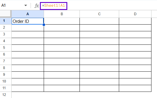
➤ Go to the destination sheet (e.g., Sheet3).
➤ Click cell A1, where you want the copied data to appear.
➤ Enter the formula:
=Sheet1!A1
➤ Press Enter, and the exact data from A1 of Sheet1 will appear instantly.
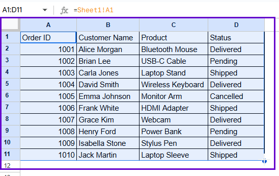
➤ Now, use the move pointer to drag it to the columns and rows to get the whole A1:D11.
Note:
You need to put the formula in one cell, not in a group of cells. If you add rows to the source sheet later, it won’t expand.
Using ARRAYFORMULA to Automatically Expand Copied Data
We want to copy new items and an entire column from the source sheet without changing the formula. When it comes to automatically expanding rows, ARRAYFORMULA excels.
Steps:
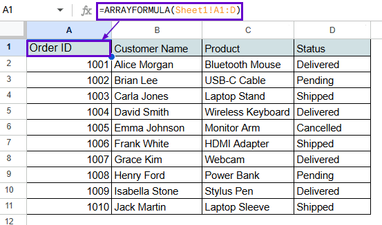
➤ Go to the target sheet, Sheet4.
➤ In the destination cell, type:
=ARRAYFORMULA(Sheet1!A2:D)
➤ Press Enter to apply the formula.
Note:
It can automatically expand as new rows are added. Make sure the structures of the columns are the same on both sheets.
Using FILTER Function for Conditional Copying
The FILTER function gives you a flexible and dynamic way to copy only certain rows based on certain conditions, such as a certain status or category. It lets you pull out and copy rows that meet certain criteria, which is amazing for making reports or putting filtered views of your data on a different sheet.
Steps:
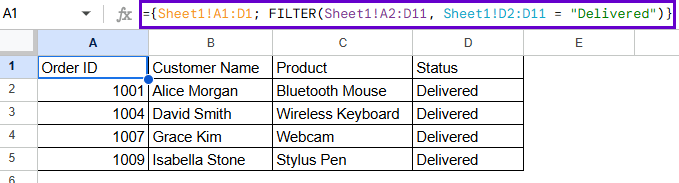
➤ Go to the target sheet, now Sheet5.
➤ Use the formula like:
={Sheet1!A1:D1; FILTER(Sheet1!A2:D11, Sheet1!D2:D11 = “Delivered”)}
➤ Press Enter, and only the rows meeting the condition will be copied.
Note:
The data range and the condition range must be the same size. This method updates right away when things change in the source sheet. Before FILTER, Sheet1!A1:D1 inside a second bracket ({}), was used to get the header of the data in Sheet1.
Using IMPORTRANGE Function
You can use the IMPORTRANGE function to automatically copy data from a different spreadsheet file, not just from a different sheet in the same file. This is very helpful when you have to deal with more than one file at once and you want to move data from one to the other in real time.
Syntax:
=IMPORTRANGE(“URL_of_Source_File”, “Sheet range”)
Steps:
➤ Open the destination spreadsheet (Sheet6) where you want to copy the data.
➤ In blank cell A1, type the following formula:
=IMPORTRANGE(“https://docs.google.com/spreadsheets/d/16TCkecFjm_UfvI0gssHfHDjNgoAnrdqapi-39Rxdleo”, “Sheet1!A1:D11”)
➤ Press Enter.

➤ The data from columns A to D will now be displayed automatically.
Note:
When you first use IMPORTRANGE in a file, you’ll get a #REF! error and a message asking you to Allow access. To let files connect, click Allow Access.
Using Google Apps Script to Copy Data Programmatically
Google Apps Script is the most effective way to copy data between sheets when you want full control over when and how it happens. It can help you decide when to click a button to start the process or set a time for it to happen. This method is great for making workflows automatic or making dashboards for teams that are easy to use.
Steps:
➤ Go to Extensions > Apps Script.
➤ Remove any code that is already there and paste the following:
function copyData() {
var ss = SpreadsheetApp.getActiveSpreadsheet();
var source = ss.getSheetByName("Sheet1");
var target = ss.getSheetByName("Sheet7");
var data = source.getRange("A1:D11").getValues();
target.getRange(1, 1, data.length, data[0].length).setValues(data);
}
➤ Click Save Project to Drive.
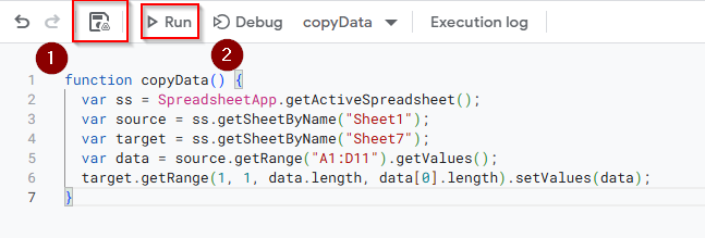
➤ Run the script by clicking the Run button and you’ll see the output as follows.
Note:
This advanced method gives you complete control; you can change the range and the conditions or even set up automatic row deletion.
Using QUERY Function to Copy Data Based on Conditions
The QUERY function works like SQL to get data and arrange it according to certain rules. If you only want to pull certain columns or filter data logically while keeping the headers, this is another great way to do it. This approach is excellent if you want a clear, filtered look at your dataset.
Steps:
➤ Select a cell where you want your result (e.g., A1 on Sheet8).
➤ Enter the formula:
=QUERY(Sheet1!A1:D11, “SELECT A, B, C, D WHERE D = ‘Delivered'”, 1)
➤ Press Enter to view only the rows where the status is Delivered.
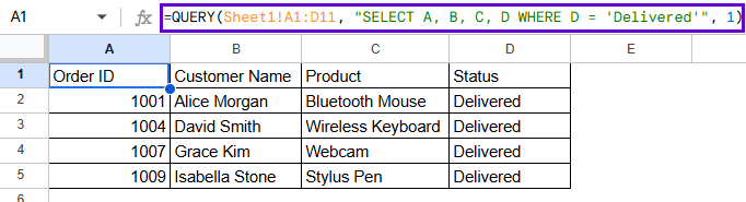
Note:
The final argument, 1, ensures the display of headers. QUERY is very flexible and easy to read, especially when it comes to making custom views of data.
Frequently Asked Questions
Can I automatically copy only new rows to another sheet?
Yes. Use FILTER with a timestamp or condition to get only new data. You can also use QUERY to filter based on new items.
Does the copied data stay updated if I change the original?
Yes, the data will update automatically whenever the original changes if you use formulas like =Sheet1!A1, ARRAYFORMULA, FILTER, QUERY, or IMPORTRANGE.
Can I automatically copy the formatting along with the data?
Unfortunately, no. The formulas in Google Sheets only copy values, not formatting. You need either Apps Script or to do it manually.
What happens if I rename the source sheet?
The formula will stop working if you change the name of the sheet it refers to. You have to change the name of the sheet in the formula by hand.
How can I stop automatic updates after copying?
To turn formulas into static values, copy the result and then choose Paste Special > Values Only. This stops the original from getting any more updates.
Concluding Words
You should now be able to confidently and quickly set up automatic data synchronizing between sheets in Google Sheets using these tips and tricks. Automating your data flow will save you hours of work that you have to do over and over again. You can make your work easier and keep your data perfectly aligned across sheets by picking the right method.