Year-to-date calculations are commonly used for budgeting, sales computations, and other data analysis purposes. If you have data for multiple years and want to sum up the data year-wise, you are at the right place. In this article, we will learn how to calculate ytd in excel so that you can perform your calculations without any difficulties.
➤ Enter this formula in the cell where you want the YTD result:
=SUMIF(B2:B13, “<=”&TODAY(), A2:A13)
➤ Replace B2:B13 with the value range and A2:A13 with the date range.
➤ Press Enter.
That was one method to do the job. But in this article, we will have four methods for you to choose from. Therefore, read the entire tutorial to become a master at calculating ytd in Excel.
What is YTD Calculation?
YTD (Year to Date) Calculation measures the data available from the beginning of the year till the current date, hence the name year-to-date. Usually, it starts from the beginning of the year and ends the moment you start calculating. For financial metrics, comparative analysis, and performance tracking, YTD calculations are very significant.
Calculating Year to Date Using SUMIF
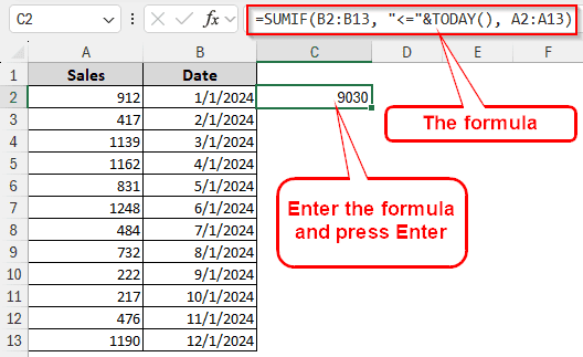
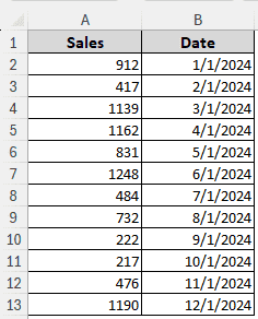
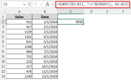
We have a set of data here with the sales figures and the dates. We are going to add up the sales data till today’s date. Complete the following steps:
➤ Write this formula in the C2 cell (that’s where we want the calculation to show up)
=SUMIF(B2:B13, “<=”&TODAY(), A2:A13)
Note:
Although it looks like the formula just summed up the sales column, it actually did that because today’s date is way past the dates in the second column. If you have a date in the date column that is past the current date, the summation will stop there. We cannot practically show that because we don’t know when you will be reading this.
Dynamic Year-to-Date Calculation Using SUM-FILTER
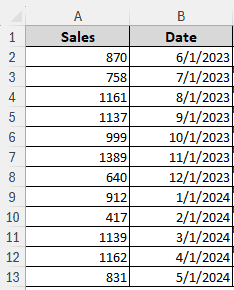
The previous method used a year-to-date calculation till the current date. But what if you needed to calculate based on predefined dates? For this example, we have a set of data with dates that start roughly in the middle of one year and end with another.
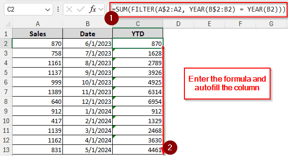
➤ Write this formula in the C2 cell so that the row matches up with the other rows:
=SUM(FILTER(A$2:A2, YEAR(B$2:B2) = YEAR(B2)))
➤ Autofill other cells.
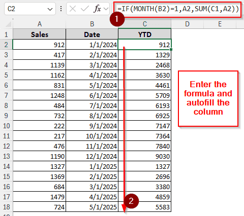
Dynamic YTD Calculation with IF-SUM
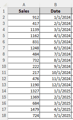
This formula is really simple and can calculate the values dynamically without any major drawbacks. This time, we will take a dataset that starts with January but goes beyond December and into the next year. Check the steps below:
➤ Like the previous method, write the formula and autofill:
=IF(MONTH(B2)=1,A2,SUM(C1,A2))
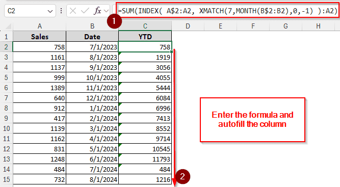
Dynamic YTD Calculation with SUM-INDEX-XMATCH
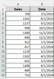
This formula works pretty much like the previous one, except it’s slower and uses way more functions. Yet we are including it because it’s good to know everything there is to know. We will be using a data set that starts with July and ends with August of the next year. Here are the steps for you to follow:
➤ You know what to do by now: insert the formula, autofill, and see the result:
=SUM(INDEX( A$2:A2, XMATCH(7,MONTH(B$2:B2),0,-1) ):A2)
Frequently Asked Questions
Can Excel automatically calculate dates?
If you are talking about filling out the dates of a column, yes, it can do that. You have to fill the first (or a few) rows so that Excel understands the pattern. Then you can use autofill to calculate the rest of the dates in the column.
How to calculate date in Excel?
There are a lot of functions to calculate dates using Excel. In the simplest format, the function DATE creates a date from year, month, and day. The formula is written like the following:
=DATE(year,month,day)
How to calculate yoy formula?
The year-over-year formula in Excel is as follows:
=(A1-B1)/B1
Here, A1 is the current year, and B1 is the previous year.
How to calculate YTD for salary?
The formula goes like this:
= ((A1/B1) – 1) *100
Here, A1 is the current year’s salary, and B1 is the previous year’s salary. The output is the percentage of salary increase for this year.
How to count dates in Excel?
Use the normal COUNT function, as Excel stores dates as numbers.
=COUNT(B1:B9)
Here, B1:B9 is the range of dates.
Wrapping Up
In this article, we learned how to calculate ytd in excel. We hope that the unique methods we used will be able to cover the usage cases you might have with year-to-date calculations. Download the workbook we used so that you can try the methods yourself without having to edit your own datasheet. Leave your feedback below, and we will see you in another tutorial.