In order to evaluate an asset and prepare for the next one, businesses need to calculate the depreciation of their properties. Among the methods of calculating depreciation, straight line depreciation is used most. In this article, we will learn the straight line depreciation formula excel with examples.
➤ Put this formula in your output cell:
=SLN(C2,D2,10)
➤ Replace C2 with the price of the asset, D2 with the salvage value, and 10 with the lifetime of the asset in years.
➤ Press Enter, and autofill other cells of the data range.
There is another formula to calculate straight-line depreciation in Excel. You might be intrigued to know about how these formulas work, and how you can do the calculation manually as well. Stick around with us and read the full tutorial to learn those in detail.
What is Straight Line Depreciation?
When you buy an asset like a refrigerator, an air cooler, or a computer, you know that the asset is not going to last forever. After some years, the machine would stop working like it’s intended, and you would have to replace it with another. Businesses do the same with their assets as well. However, as everything needs to go through a process in a business, they calculate the depreciation of their assets so that they can have the money to replace the product after a certain period of time.
Among all the other methods of calculating depreciation, the straight-line method is the most straightforward. An asset, even if it breaks, has a salvage value. In the straight line depreciation method, the salvage value is subtracted from the cost of the machine, and the rest of the value is divided among the time period the machine will be used. In this tutorial, we will do that calculation in Excel.
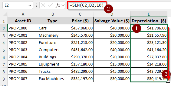
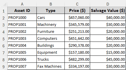
For this example, we have a dataset with some asset IDs, the asset types, their prices, and salvage values. We are going to calculate the straight line depreciation of those assets using the prices and the salvage values. All of the assets in the data range are supposed to last for 10 years. Let’s see the calculation in action.
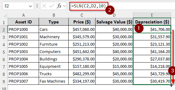
Using the SLN Function to Calculate Straight Line Depreciation
Excel provides us with a straightforward function that can be used to calculate straight-line depreciation. Here is how to do that:
➤ Use an output column for the depreciation. We are using the E column for this.
➤ Write this formula in the E2 cell:
=SLN(C2,D2,10)
➤ After pressing Enter, use your mouse to drag the cell to autofill the whole column.
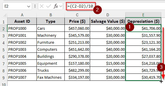
Calculating Straight Line Depreciation Manually
Instead of using the function excel provided, we can use the regular mathematical expressions and calculate the depreciation manually. Follow the steps below to learn the method:
➤ Use an output column for the calculation:
➤ Copy this formula and change the cell references from your dataset:
=(C2-D2)/10
➤ Fill the other cells using autofill by clicking and dragging your mouse.
Frequently Asked Questions
What is the difference between the sln and db method of depreciation?
In the DB, or declining balance method, the depreciation rate is the same for the lifetime of the asset. While SLN uses the same amount for the lifetime, DB uses a percentage rate that is subtracted from the previous year’s value of the asset. As a result, the depreciation amount becomes different for each year.
Which depreciation method is best?
There is no best method for calculating depreciation. The best method for calculation will depend on your dataset and usage case. However, the straight-line depreciation method is the most commonly used.
How to calculate residual value?
Even after an asset is ready to be salvaged, there is a cost of scraping the material. Residual value is the amount that remains after subtracting the salvage cost from the salvaged value.
What is syd in Excel?
SYD is another function for calculating depreciation in Excel. This function is used for calculating using the sum-of-years method. It is mostly used for fixed assets. The syntax of the function is as follows:
=SYD([Cost],[Salvage],[Life],[Per])
Where is depreciation in P&L?
Depreciation is a cost to the company, and it is debited in the profit and loss statement. In the balance sheet, the amount of depreciation is deducted from the asset.
Wrapping Up
In this article, we learned two ways to calculate straight-line depreciation in Excel. We hope that you will be able to utilize the straight line depreciation formula we used in this tutorial. Download the workbook to practice the method yourself without harming your existing workbooks. Consider leaving your feedback below, and we will see you in another tutorial.