How to Flip a Table in Excel (8 Suitable Ways)

Flipping a table in Excel mostly refers to two things: reversing the data order upside down or swapping columns and rows. Excel doesn’t offer direct functions or features for either, so we need to apply some tricks and combine functions to flip a table.

To flip data order, we’ll add a helper column with sequential numbers and sort them to largest to smallest value. For column and row rotation, we’ll use the transpose feature to flip the table while copying it.

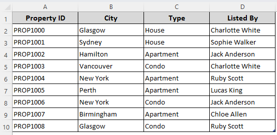
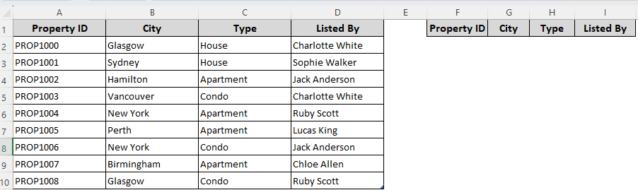
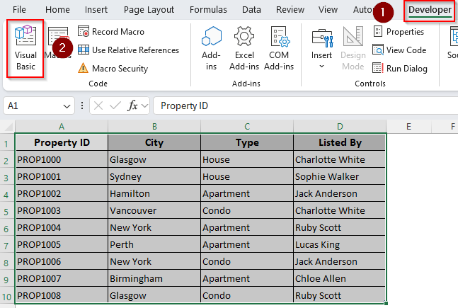
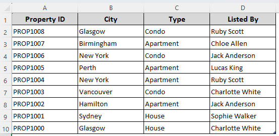
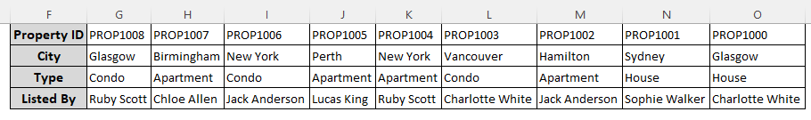
To demonstrate the methods, we’ll use a dataset featuring real estate listings with columns for property ID, city, type, and listing agent name. We’ll reverse the data order within the table and swap the columns and rows.

Although sorting alphabetically doesn’t flip table data, sorting data from largest to smallest based on sequential numbers solves the problem. Therefore, we’ll add a helper column to sort our data. Below are the steps:

➤ Create a helper column and enter the numbers 1,2,3…. in each subsequent cell. You can type 1 and 2 in the first two cells and use the fill handle (+ sign) to autofill the rest.
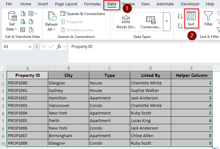
➤ Select your entire data range and open the Data tab from the top ribbon. Click on Sort from the Sort & Filter group.

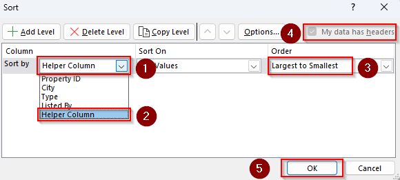
➤ As the Sort box appears, click the Sort By drop-down and choose the helper column header.
➤ In the Order field, choose Largest to Smallest. Make sure the My Data Has Headers box is checked.

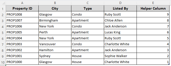
➤ Press Ok and the data order is now flipped. You can keep the helper column or delete it after the data order is flipped.

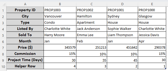
For this method, we’ll change the positions of our rows and columns. Creating a helper row and sorting it will flip our table data. Below are the steps:

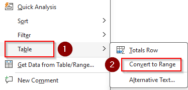
➤ First, right-click on your data range and select Table >> Convert To Range from the menus. Excel doesn’t allow sorting from left to right for filtered tables.

➤ Create a helper row and fill it with sequential numbers (1,2,3….).
➤ Highlight your data range and open the Data tab >> Sort.
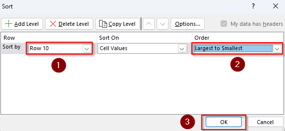
➤ From the Sort dialog box, Click on Options, choose Sort Left to Right from the Sort Options dialog box, and press Ok.

➤ Now, click on Sort By and select the row number where you created the helper row.
➤ Choose Largest to Smallest from the Order drop-down and click Ok.

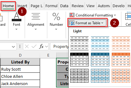
➤ As Excel flips the data from right to left, you can format your data range back as a table by going to the Home tab >> Format As Table. Here’s the final result:

In Excel 365/2021, the SORTBY function sorts a range or table based on the values in another range or array in ascending or descending order. With the ROW function, we’ll sort our table based on its rows in descending order.

However, the sorted output is placed in a different location. Here are the details:

➤ First, choose a location to put the table with the flipped data. Copy and paste the column headings in your chosen location.

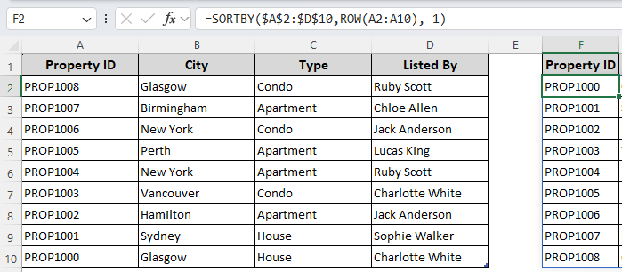
➤ In the first column cell, enter the following formula:

➤ Replace $A$2:$D$10 with the column range of your original data without the heading. Instead of A2:A10, enter the row range. Here, -1 indicates that we want the data in descending order.
➤ Finally, press Ok. Copy the values with the Paste Special option on your original table.
➤ For this, select your data range and right-click on the selection. Choose Paste Special and select Values from the Paste Special dialog box.

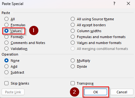
➤ Click Ok and you’ll get the flipped table like the one displayed below:

For older Excel versions, you can use the INDEX function which returns a value from a table or range based on row and column numbers. To define the location of the columns and rows, we’ll combine it with the ROWS and COLUMNS functions. Follow the steps below:

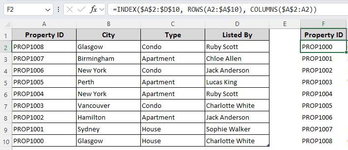
➤ Select a location to enter the flipped dataset and copy the headers. In the first cell of the new location, enter this formula:

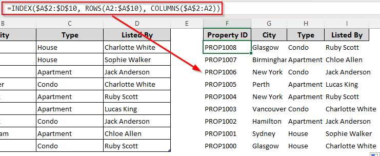
➤ Click Ok and drag the formula down the column and across the rows using the fill handle.
➤ Finally, copy the values with the Paste Special option on your original table. Here’s the final result.

Creating a custom VBA macro offers greater control over large and complex datasets. Let’s apply codes that flip table data by columns (vertically) or by rows (horizontally). You can also choose to transpose the table to swap columns and rows.

Steps:

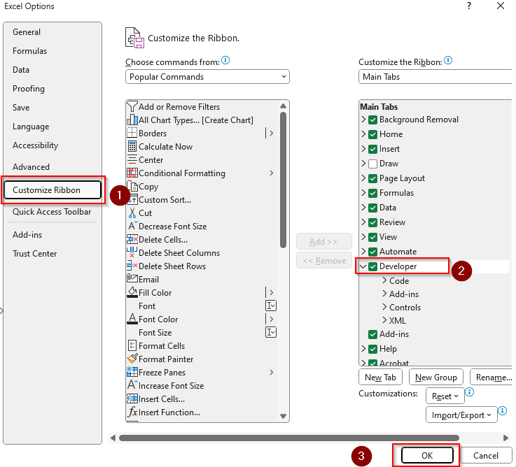
➤ To add the Developer tab in your top ribbon, go to the File tab >> More >> Options.

➤ Select Customize Ribbon and check the Developer box. Press Ok.

➤ Select your entire table without the headers and open the Developer tab. Click on Visual Basic.

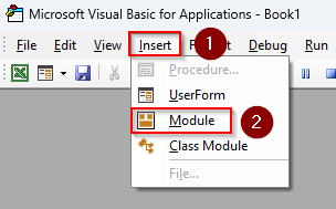
➤ Select the Insert tab and click on Module.

➤ In the new module box, enter the following code:

Sub FlipOrTransposeRange()
Dim rng As Range
Dim optionChoice As String
Dim r As Long, c As Long
Dim outRng As Range
Dim tempArr As Variant
Dim newArr() As Variant
' Prompt user for selection type
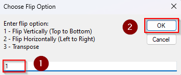
optionChoice = InputBox("Enter flip option:" & vbCrLf & _
"1 - Flip Vertically (Top to Bottom)" & vbCrLf & _
"2 - Flip Horizontally (Left to Right)" & vbCrLf & _
"3 - Transpose", "Choose Flip Option")
If optionChoice = "" Then Exit Sub ' Cancelled
Set rng = Selection
If rng Is Nothing Then
MsgBox "Please select a range first.", vbExclamation
Exit Sub
End If
tempArr = rng.Value
Select Case optionChoice
Case "1" ' Flip Vertically
ReDim newArr(1 To UBound(tempArr, 1), 1 To UBound(tempArr, 2))
For r = 1 To UBound(tempArr, 1)
For c = 1 To UBound(tempArr, 2)
newArr(r, c) = tempArr(UBound(tempArr, 1) - r + 1, c)
Next c
Next r
Case "2" ' Flip Horizontally
ReDim newArr(1 To UBound(tempArr, 1), 1 To UBound(tempArr, 2))
For r = 1 To UBound(tempArr, 1)
For c = 1 To UBound(tempArr, 2)
newArr(r, c) = tempArr(r, UBound(tempArr, 2) - c + 1)
Next c
Next r
Case "3" ' Transpose
ReDim newArr(1 To UBound(tempArr, 2), 1 To UBound(tempArr, 1))
For r = 1 To UBound(tempArr, 1)
For c = 1 To UBound(tempArr, 2)
newArr(c, r) = tempArr(r, c)
Next c
Next r
Case Else
MsgBox "Invalid option selected.", vbExclamation
Exit Sub
End Select
' Clear original range and resize for output
Set outRng = rng
If optionChoice = "3" Then
Set outRng = outRng.Resize(UBound(newArr, 1), UBound(newArr, 2))
End If
outRng.ClearContents
outRng.Value = newArr
MsgBox "Operation completed successfully.", vbInformation
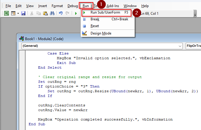
End Sub

➤ Click on the Run tab and choose Run Sub/UserForm from the menu. Or, press the  F5  key.

➤ Go back to the Excel tab and select whether you want to flip the table vertically, horizontally, or transpose it. Press Ok.

➤ Excel will now change the table order based on your selection.

➤ While closing the file,  Excel prompts you to save the changes. Make sure you save the file correctly.

For some users, flipping a table means swapping the columns and rows. Commonly referred to as transposing, here, the data from rows converts into columns and vice versa.

In this method, we’ll rotate or transpose the table to a different location on the worksheet. Let’s get to the steps:

➤ As the Transpose option isn’t available for filtered tables, we need to change our table data into range. For this, highlight your table and right-click on it. Select Table and click on Convert To Range.

➤ Select your entire table’s dataset and press the  CTRL  +  C  shortcut key to copy it. Or, right-click on the selection and choose Copy from the menu.
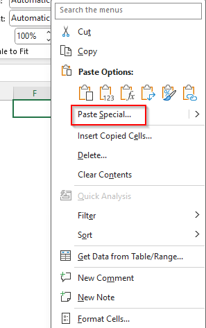
➤ Choose a location in your worksheet to put the flipped/transposed data. Right-click on the first cell to start the flipped table and select Paste Special from the menu.

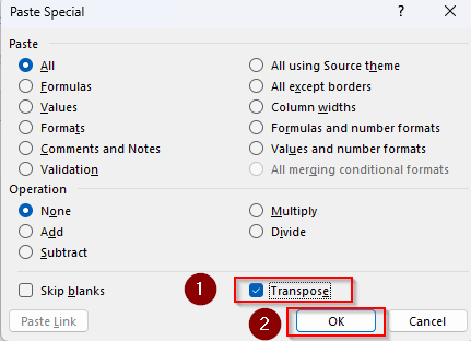
➤ From the Paste Special dialog box, check the Transpose box and press Ok.

➤ Now, your table is flipped with the data from the rows transformed into the columns and vice versa. To turn the flipped range into a table, go to the Home tab and select Format As Table. Choose your preferred table format.

➤ Here’s our final data:

To use the TRANSPOSE function, we’ll create an array formula that switches the locations of your table rows and columns. The step-by-step procedure is as follows:

➤ Choose a location where you want to input the flipped dataset. Make sure you have enough space to accommodate all the converted rows and columns.
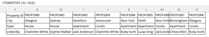
➤ In the first cell where you want to start the flipped table, enter the following formula:

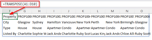
➤ Replace A1:D10 with your original table range including the headings.
➤ For Excel 2019 or newer versions, press Ok to enter the formula. If you’re using an older version, press the  CTRL  +  SHIFT  +  ENTER  keys to enter the array formula.

For dynamic changes that apply to future entries, we use the Power Query tool. Here’s how to use it to rotate a table and enter the flipped table in a new worksheet:

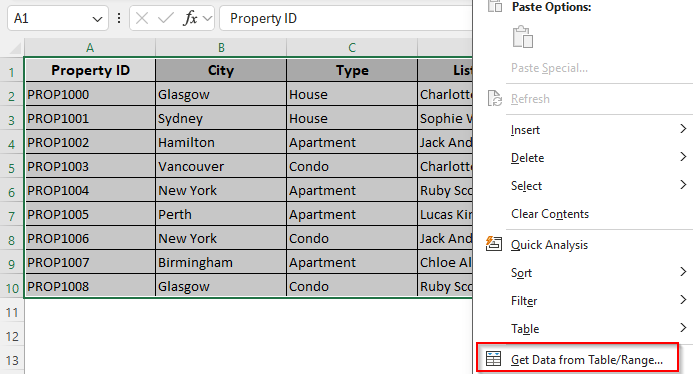
➤ Select your entire table and right-click on the selection. Choose Get Data From Table/Range from the menu.

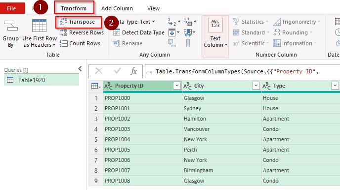
➤ In the Power Query Editor, select the entire table, go to the Transform tab, and click on Transpose.

➤ Once the table is flipped, open the Home tab and select Close & Load.
➤ As Excel loads your table in a different worksheet, make necessary changes in the table format using the Table Design tab.

Frequently Asked Questions

Can you flip a shape in Excel?

Yes, you can flip a shape in Excel. To flip a shape, select your shape and click on the Shape Format tab. Press the Rotate button in the Arrange group. Now, choose Flip Horizontal to mirror the shape left to right. Or, select Flip Vertical to mirror the shape top to bottom.

How to flip text horizontally in a cell in Excel?

Select the cell with the text you want to flip and go to the Home tab. From the Alignment group, click on Orientation. Now, select any of the given options as needed to rotate the text up, down, vertically, clockwise, or counterclockwise.

How do you quickly flip signs in Excel?

To flip the sign (positive to negative or vice versa), select a cell to put the flipped sign and insert the following formula:
=A1 * -1
Here, A1 is the cell containing the original sign. Change the cell reference based on your data. Press Enter.

Concluding Words

Whether you want to reverse the data order of your table or swap the positions of columns and rows, we’ve covered everything you need to flip a table in Excel. Using the SORTBY function and the Transpose feature is the easiest way for both tasks.
However, for more flexibility and large datasets, using the Power Query tool and VBA coding is preferable to reduce potential errors.