
The VLOOKUP function in Google Sheets is a helpful tool for searching and retrieving information from a specified range, whether it is within the same or different spreadsheets. It allows users to pull and extract information across different sheets for better data analysis and reporting. You can use multiple methods to perform a VLOOKUP operation by using Google Sheets’ built-in tools.
To use VLOOKUP for retrieving information from another worksheet, follow the steps below:
➤ Open your spreadsheet file.
➤ Select the cell that you want to perform the VLOOKUP operation, and put the formula:
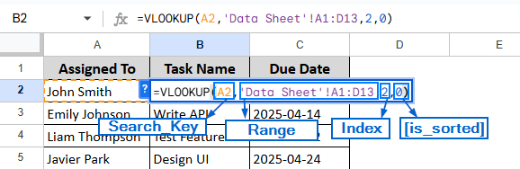
=VLOOKUP(search_key, range, index, [is_sorted]).
➤ Replace “search_key” with the cell whose value you want to search.
➤ Replace “Range” with the range of cells or columns containing the data, including the sheet name from where you’re fetching data.
➤ Replace “Index” with the column number from which to return the value.
➤ Replace “[is_sorted]” with 0 or 1. Here, “0” indicates an exact match and “1” indicates an approximate match.
In this article, we will learn 2 easy methods of using VLOOKUP from another sheet in Google Sheets.
Use VLOOKUP in the Same Spreadsheet Across Different Workbook
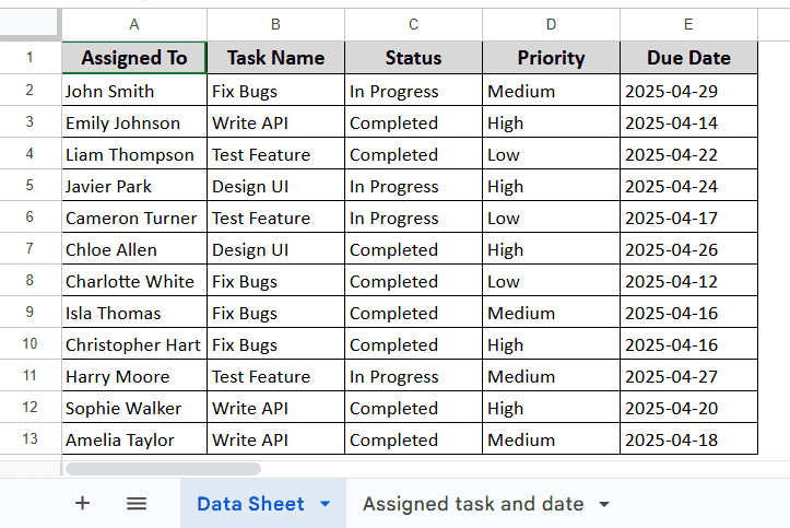
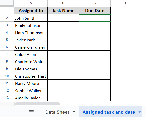
This method is particularly useful for searching data within the same spreadsheet distributed across multiple sheets. In the sample dataset, we have two sheets. One containing all the necessary information, including who the task is assigned to, the task name, status, priority and due date. We will name this sheet as Data sheet. And in the second sheet, called Assigned task and date, we only have information about who the task is assigned to. Using the VLOOKUP function, we have to find out their task name and Due date.
Steps:
➤ Open the spreadsheet.
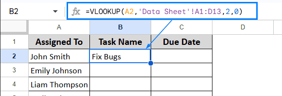
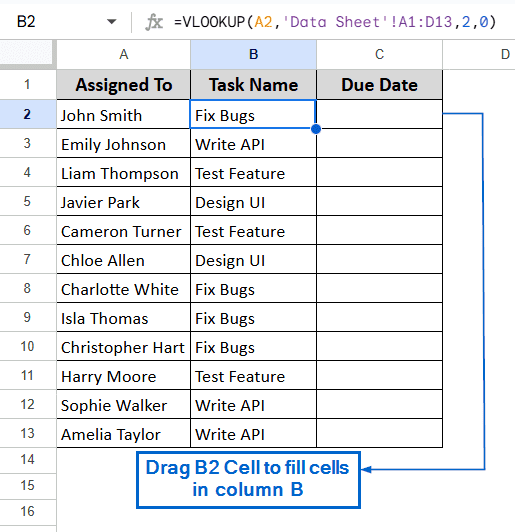
➤ In the Assigned task and date sheet, select the B2 cell and put the formula:
=VLOOKUP(A2,’Data Sheet’!A1:D13,2,0)
Note:
In the formula, “A2” refers to the value to search for. In our case, it is the name of the person whose task we need to find. “’Data Sheet’!A1:E13” specifies the name of the sheet and the range. Since the Task Name is located in the second column of that range, we use “2” to tell the formula which column to return the result from. And lastly, the value “0” indicates that we want an exact match for the value in the A2 Cell.
➤ Next, press Enter, and drag B2 cell to fill the Task Name column with the task assigned to each person.
Note:
Instead of manually dragging the cell to fill the column, you can also use the Auto-fill feature.
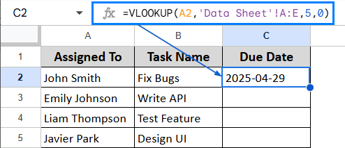
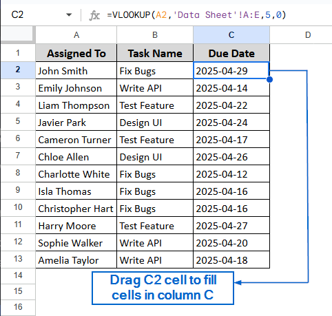
➤ Again, select the C2 cell this time to find out the Due Date and put the formula:
=VLOOKUP(A2,’Data Sheet’!A:E,5,0)
➤ Hit Enter, and drag C2 cell to fill the Due Date column. Now you have successfully found out the task name and the due date assigned to each person.
Use VLOOKUP Between Different Workbooks Using IMPORTRANGE
The IMPORTRANGE function is used to import a range of cells or columns from an entirely different spreadsheet into your current one. This function is particularly helpful when you need to retrieve information using VLOOKUP from a completely different spreadsheet file. In this example, we will work with two separate spreadsheets. The first one contains all the necessary information about the task name, who the task is assigned to, status, priority and due date. The second spreadsheet only lists the names of the people assigned to tasks. Our goal is to pull the Task Name and Due Date from the first spreadsheet into the second one using the VLOOKUP and IMPORTRANGE functions. Follow the steps below to properly do it.
Steps:
➤ Open the first spreadsheet file containing the Data Sheet sheet.
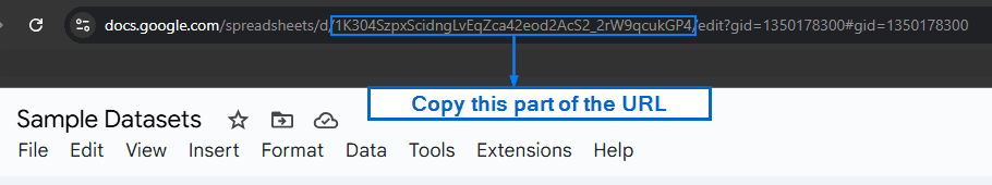
➤ From your browser, copy the URL of the file.
Note:
No need to copy the entire URL. Only copy the parts between d/ and /edit.
➤ Now, head to the second spreadsheet and in the B2 cell, put the formula:
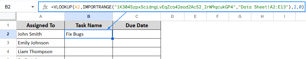
Note:
“1K304SzpxScidngLvEqZca42eod2AcS2_2rW9qcukGP4” within the IMPORTRANGE function represents the URL of the source file. All the other parts of the formula have already been explained in the first method.
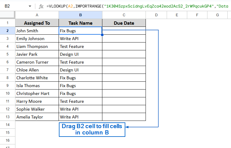
➤ Press Enter and drag B2 cell to fill the Task Name column.
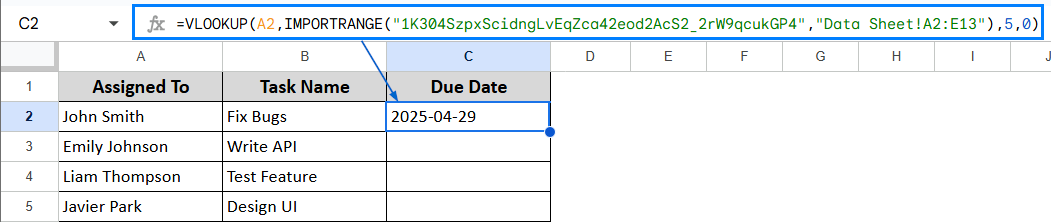
➤ Again, head to the C2 cell and put the formula:
=VLOOKUP(A2,IMPORTRANGE(“1K304SzpxScidngLvEqZca42eod2AcS2_2rW9qcukGP4″,”Data Sheet!A2:E13”),5,0)
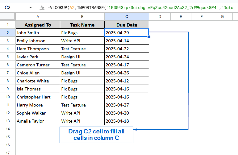
➤ Hit Enter and drag C2 cell to fill Due Date column.
Frequently Asked Questions
Why is VLOOKUP returning #REF! Error?
#REF! Error mainly occurs when the column index number exceeds the number of columns in the lookup range. It can also happen because of incorrect sheet name, rogue spaces and invalid URL.
Can I Use VLOOKUP On a Different Google Sheets File?
Yes, you can use VLOOKUP with the help of the IMPORTRANGE function to import data from a different spreadsheet file. The process has already been discussed in the second method.
Why is VLOOKUP returning #N/A Error?
If VLOOKUP is returning #N/A error, it means the value you are searching for was not found in the specified lookup column. This error can also happen if you have extra spaces or mismatched data types.
Concluding Words
Using VLOOKUP to retrieve data across different sheets is a smart and efficient way to manage datasets and streamline workflows. In this article, we talked about 2 useful methods of using VLOOKUP to extract information from spreadsheets, including using VLOOKUP between sheets within the same spreadsheet, and using it across two separate spreadsheets with the help of the IMPORTRANGE function. Feel free to try out both methods and choose the one that best fits your needs.