A legend is a section of the chart that represents the meaning of different colors, lines, shapes, etc. It works as a visual guide for understanding each series better. Editing a legend in excel means modifying its text, position, order, and appearance, or removing specific entries to improve clarity and presentation in a chart.
By default, Excel creates a chart with its default color theme. The legend position is random depending on the chart and source data (from where you plot the chart).
Moreover, if you don’t select the proper headers, it can add its own name to the labels.
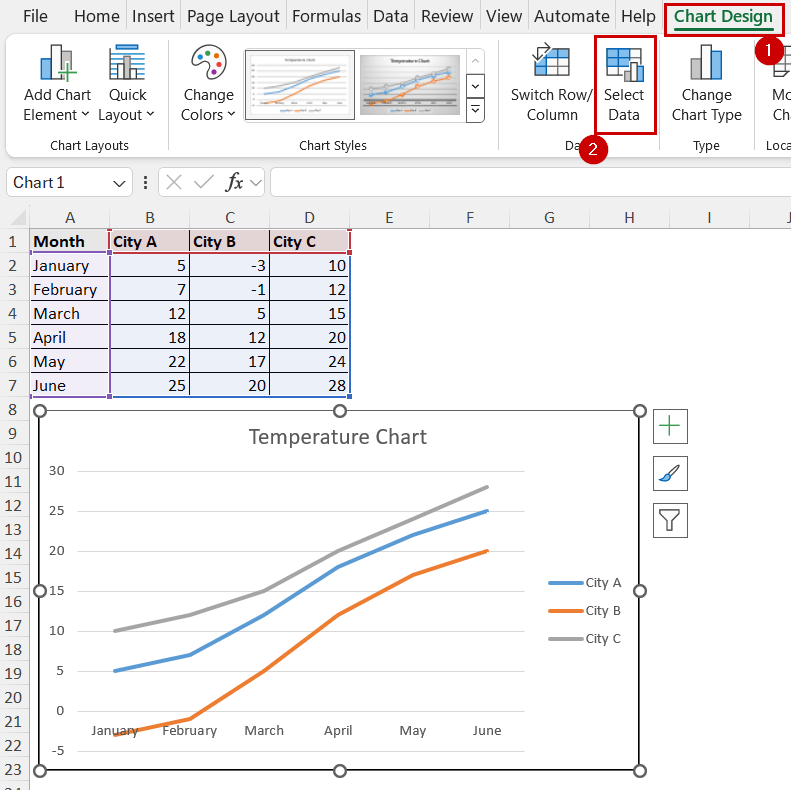
➤ Change the text of the legend in the Edit Series box. You can access that from the Chart Design >> Data (group) >> Select Data.
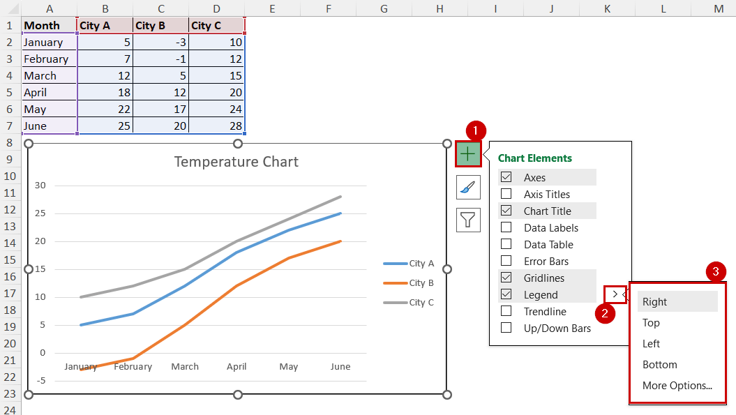
➤ You can move the legend position on the chart by selecting Chart Element >> Legend >> then selecting the position.
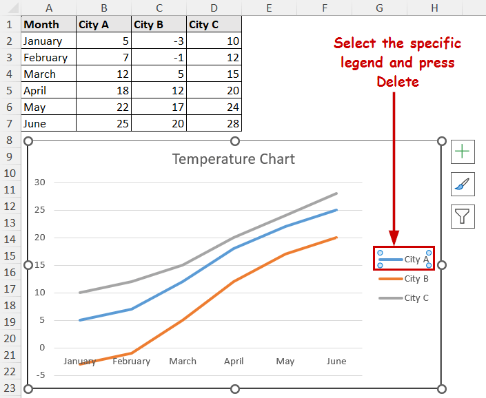
➤ You can remove a specific legend by selecting that one only and pressing the Delete button.
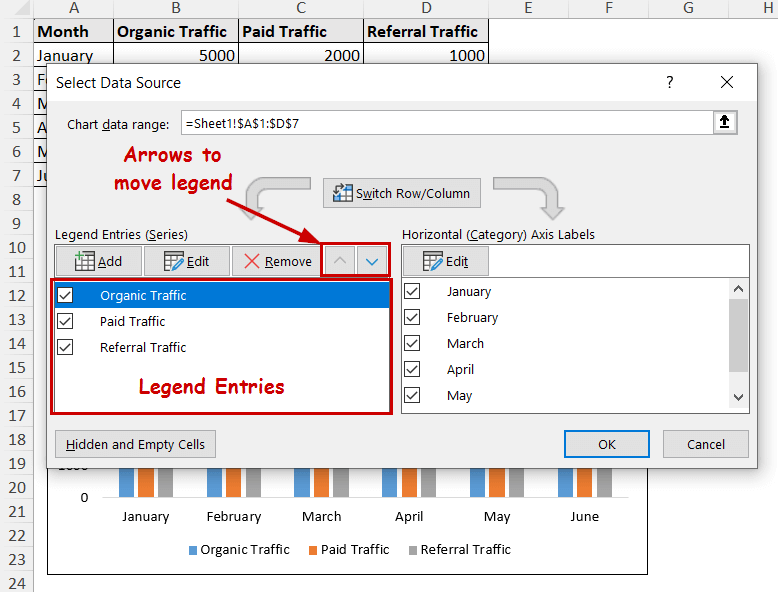
➤ The Select Data option from the Chart Design tab also offers how you want to keep the legend’s order.
➤ You can access different formatting options of the legend text and the legend area by right-clicking on the legend and selecting Format Legend from the context menu.
While Excel’s default chart is workable in most cases, they are not the best when it comes to representations. They can be a bit tedious to understand in some cases. The chart doesn’t serve its core purpose in those cases.
In this tutorial, we will go through how you can edit the default legend styles in Excel. We will cover all the types of edits you can perform in the legend.
Download Practice WorkbookChanging Text of Legend
Excel usually includes data headers as legends. When you don’t have such headers, it creates series 1, 2, etc.
You may face the latter situation more often to edit a legend. Or, you may feel other descriptions suit you better. The existence of legend is to clarify and improve the understandability of a chart after all.
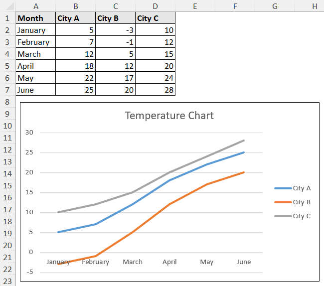
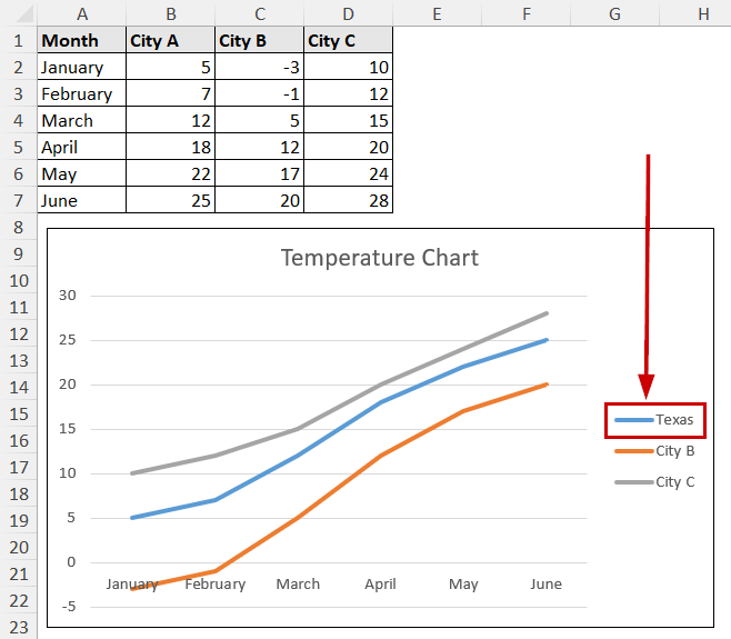
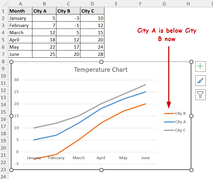
Before we dive into how we can change the text, let’s look at our dataset.
It contains temperatures of different cities across different months. We have plotted this data in a line chart with legends indicating which line belongs to what city.
Steps:
➤ Select the chart by clicking on it.
➤ Go to Chart Design >> Data (group) >> Select Data.

➤ In the Select Data Source box, select the series in the Legend Entries section and click on Edit.
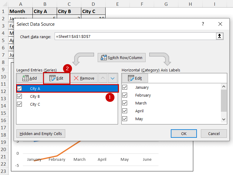
➤ Then change the Series name to the new text in the Edit Series box.
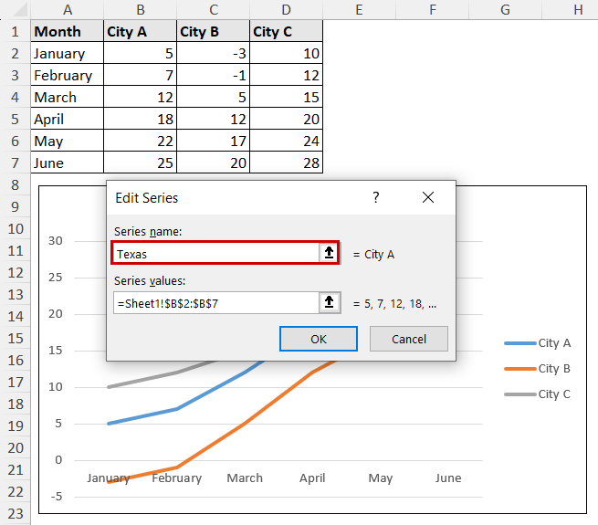
➤ Click on OK in both boxes to close them.
The legend’s text will get updated this way.
Moving Legend in Chart
Excel has four primary positions (left, right, top, and bottom) for legends. It also automatically assigns the position when you create the chart or add a legend.
However, the default position may not suit the chart always. Here’s how you can change that:
Steps:
➤ Select the chart.
➤ Click on the Chart Elements button.
➤ Click on the right arrow beside the Legend option.
➤ Select the position you want from the list.
Alternative Method: You can change the position using the Chart Design tab too. It appears on the ribbon after you select the chart.
Go to Chart Design >> Chart Layouts (group) >> Add Chart Element >> Legend >> then select the position.
Remove a Specific Legend Entry
Excel, by default, shows the legend for all the series in a chart. To focus on the important ones (or to remove an unnecessary one), you need to keep some of it and delete some.
Steps:
➤ Click on the specific legend you want to delete.
➤ Press the Delete button on your keyboard.
Customizing Legend Order
The legends in an Excel chart usually maintains the order of the source data. However, you may want to change that order in the graph to improve the presentation, or grouping similar data types, etc.
In this section, we are going to show you how to change the legend order in an Excel chart.
Steps:
➤ Start by selecting the chart and go to the Chart Design tab.
➤ Go to Data (group) >> Select Data.
➤ Now select a legend from the Legend Entries section of the Select Data Source box.
➤ Move the entry up or down using the upward or downward arrows above it.
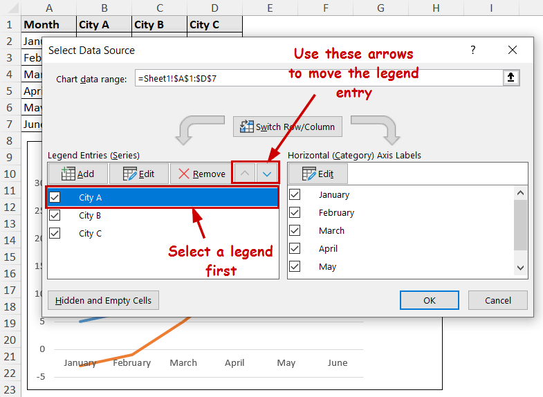
➤ Click on OK after you are done customizing each entry. The legends will get arranged in the order you assemble here.
Formatting Legend Appearance
You can also treat legends like text objects in Excel. That includes formatting the texts, adding borders, changing font, styles, etc.
You can do all of these in different methods too. Regardless, Excel has all the options included in the Format Legend window.
You can access this window by the following steps.
Steps:
➤ Right-click on a legend.
➤ Select Format Legend from the context menu.
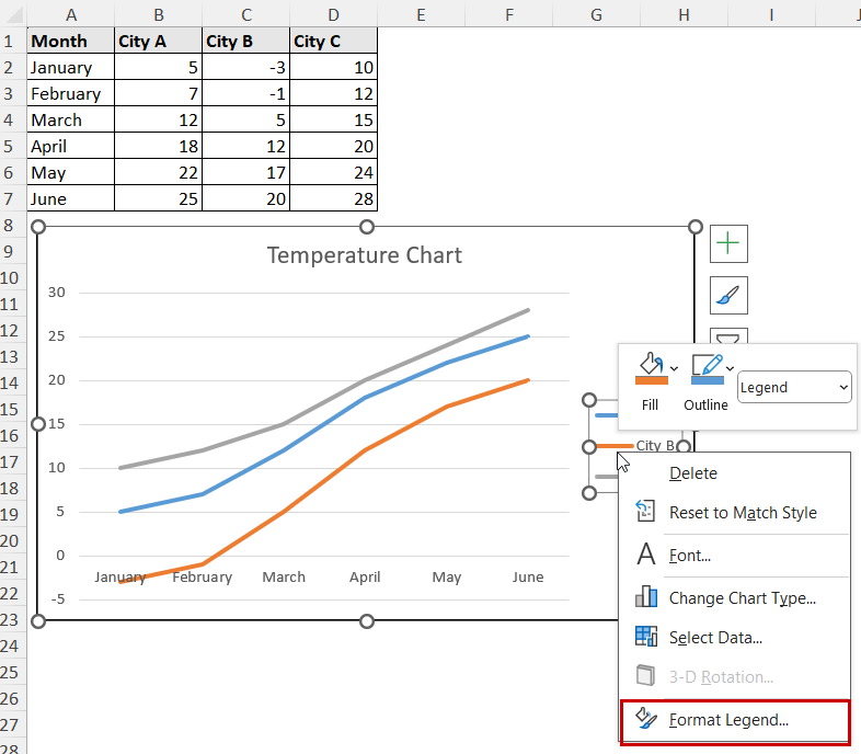
The Format Legend window will now appear on the right of the spreadsheet.
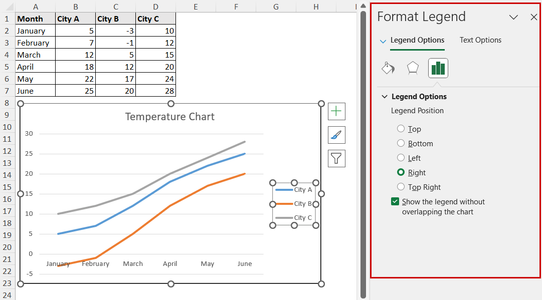
You can access all the edit options of the legend from here.
FAQ
How do I change the series 1 name in Excel?
The “Series 1”, “Series 2”, etc. appear in the legend name when the source data doesn’t have any label for a column or row, or the user doesn’t select them. You can change those using the first method described in this article.
How to customize the symbols or colors in the legend?
The colors of the legend always indicate the color of the series. You can change a series’ color by changing it’s fill after selecting it. The legend will automatically reflect that.
Why are my legend entries showing as “Series 1,” “Series 2,” etc.?
This happens when you don’t select the headers when creating the chart. Or you simply don’t have any headers in a dataset. Add headers from the Select Data options from the Chart Design tab, or add custom names for the series (if you don’t have headers) from the same option.
Why are some legend entries missing in my chart?
Legend entries can go missing because of hidden or filtered data, or not selecting the data properly. Make sure to change the source to full data while all data are showing to display them all.
Wrapping Up
In this tutorial, we have covered different types of edits of the legend in an Excel chart.
This includes changing and editing the text, moving legend positions, customizing the legend order, and removing legends.
Feel free to download the practice file and let us know about your feedback.