How to Create Outside End Data Labels in Excel (3 Quick Methods)

Data labels are text boxes that appear next to or on top of data points in the chart. “Outside end data labels” in Excel means the outside positioning of data labels that are just at the edge of the boundary.

Data labels show details such as data values, series, percentages, and other relevant information. They make the charts easier to understand.

Outside-end data labels do not overlap with the chart area, so they make the charts clearer.

There are three methods to create data labels in the outside end in Excel.

In this article, we are going to cover how to create outside end data labels using the Chart Elements button, Chart Design tab, and the context menu.

The Chart Elements button is the plus icon that appears at the top-right after selecting a chart.

It allows users to add, modify, or remove different elements quickly. Data labels and their positions are one of the elements that can be accessed from the button.

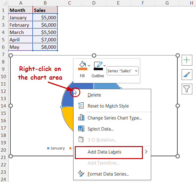
Let’s say we have the following data containing sales across different months.

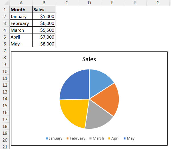
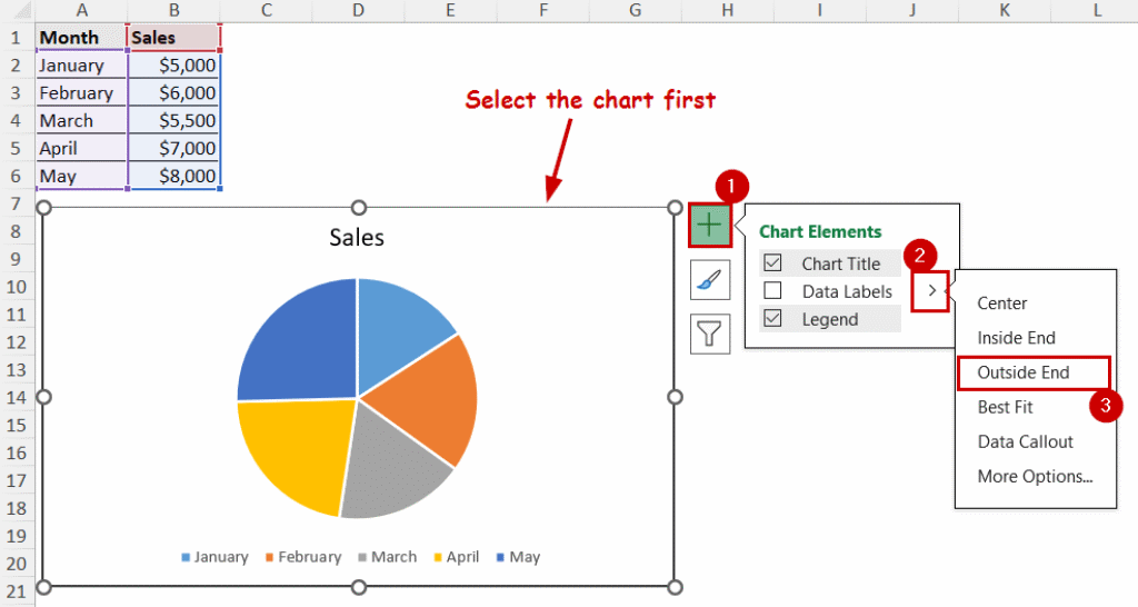
We are going to use the Chart Elements button to add outside end data labels in the pie chart we have created from the data.

Steps:

➤ Select the chart.
➤ Click on the Chart Elements button (the plus icon at the top-right).
➤ Then click on the right arrow beside the Data Labels option.
➤ Select the Outside End option as the position.

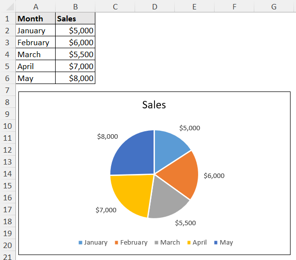
The chart will now have outside end data labels.

After selecting a chart, two additional tabs are accessible in the ribbon: Chart Design and Format. You can add different elements from the Chart Design tab. These elements include data labels and their positions.

Steps:

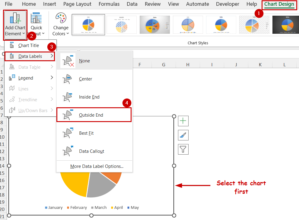
➤ Select the chart.
➤ Go to Chart Design >> Chart Layouts (group) >> Add Chart Element.
➤ Select Data Labels from the dropdown.
➤ Then select Outside End.

This will also result in the same outside-end data label position.

The two methods access the same options in two different ways.

You can also add data labels from the context menu. With the Format Axis pane, you can edit their positions to move them to an outside end later.

Steps:

➤ Right-click on a chart area containing the series. (the pie in our chart)
➤ Select Add Data Labels from the context menu.

➤ Now right-click on the same chart area again.
➤ Select Format Data Labels from the context menu this time.

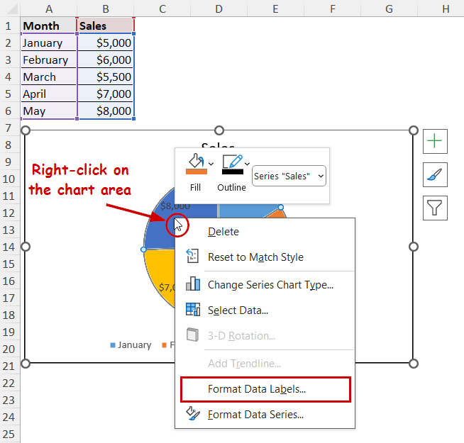
The Format Data Labels pane will now open on one side of the sheet.

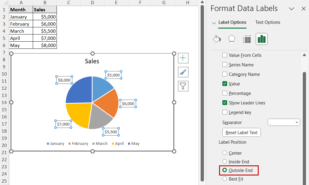
➤ In the Format Data Labels pane, select Outside End under the Label Position.

FAQ

Why are my Excel data labels not showing at the outside end?

For some chart types, such as stacked columns, the outside end position for data labels isn’t available. You have to change the chart type or the label position.

How do I hide outside end data labels in Excel?

Hiding outside-end data labels is the same as hiding any other positioned data labels. Click on the chart elements button and uncheck the data labels from there to hide the data labels.

How do I align outside end data labels to avoid clutter in Excel charts?

You can move the data labels even after selecting a position. You can align them manually to your desired position. The chart also needs to be large enough to avoid clutter.

Wrapping Up

In this article, we have covered how to add outside-end data labels in Excel. We have used the Chart Elements button, Chart Design tab, and context menu to do so.

All of the methods access the same options in different ways, you end up with the same result. The context menu one also requires the Format Data Labels pane. However, both the options are still the same.

Feel free to download the practice workbook and give us feedback.