Trend analysis is the method of identifying patterns or data shifts over time. To calculate trend analysis, Excel provides different features and functions.
In trend analysis, the main goal is to measure the direction of data. It is helpful to evaluate performance, forecast future trends, and make an informed decision based on the data. Its application is dominant in business, finance, science, healthcare, and almost all data-driven fields. With Excel’s built-in features and accessibility, it is a great tool to calculate trend analysis.
To calculate trend analysis in Excel:
➤ Use the following formula in the output cell:
=TREND(y-values,x-values)
➤ Both x-values and y-values have to be within the ranges of the independent and dependent variables.
➤ Press Ctrl + Shift + Enter to get the values.
➤ Plot the output values and previous y values in a line chart for a trend comparison.
In this tutorial, we are going to share three main ways to calculate trend analysis in Excel. In doing so, we’re going to cover finding the trendline equation and interpreting the equation, using the TREND and FORECAST functions to calculate the trend directly.
Download Practice WorkbookDisplaying Trendline from Charts
Excel charts can display the overall trendline and the trendline equation. However, you need the source data plotted in a chart to display the trend. Not all charts can fit a trendline either. So, you have to pick one that can display trendlines.
We have the following data of test scores with the hours studied for it, and we have plotted a scatter plot to demonstrate the method.

Steps:
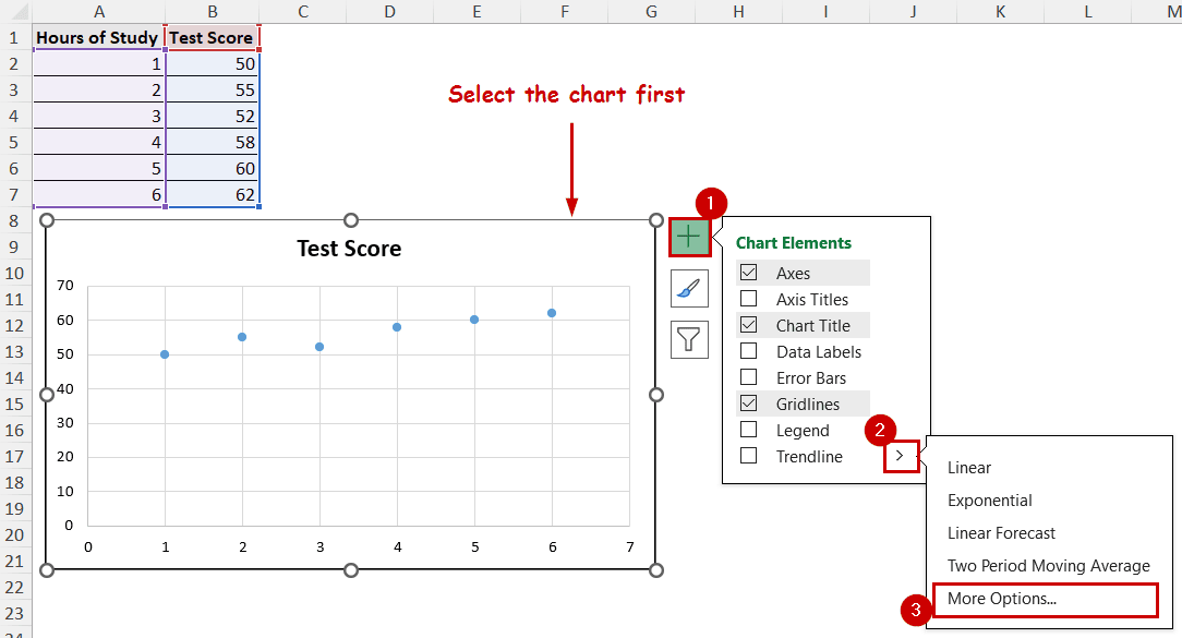
➤ Select the chart.
➤ Click on the Chart Element button on the top-right of the chart.
➤ Then click on the right arrow beside Trendline and select More Options.
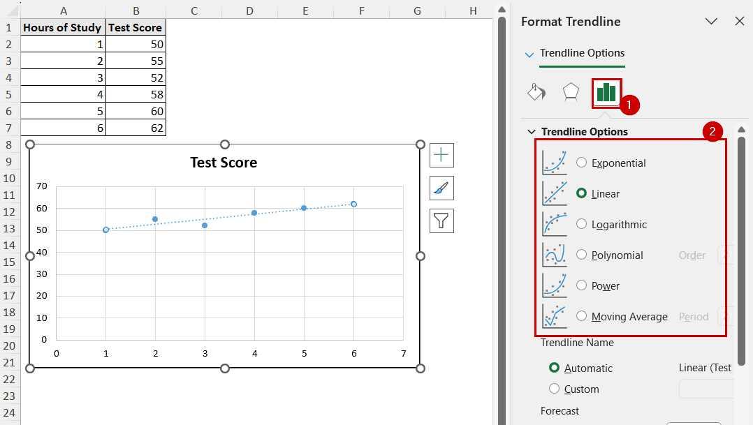
➤ In the Format Trendline pane, select a suitable trendline type.
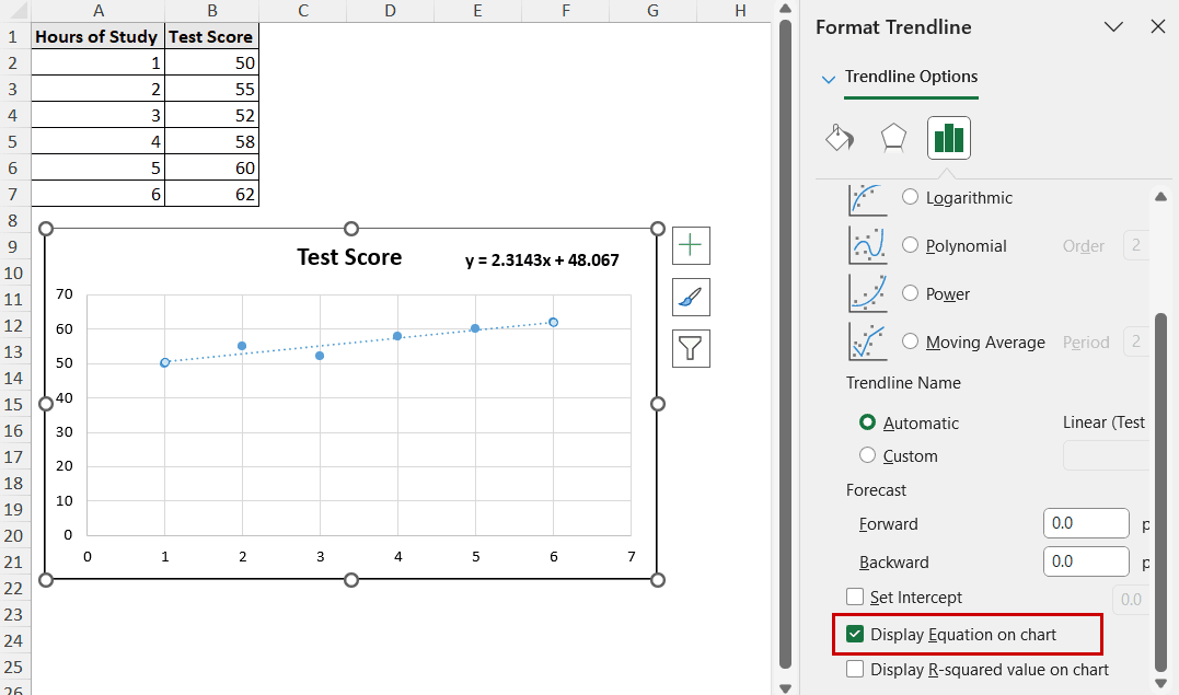
➤ Under the same options, select Display Equation on chart.
Note: You can select a trendline type directly from Chart Elements. In that case, double-click on the trendline to open the Format Trendline pane.
Trend Calculation:
From the equation, we can see it has a slope of 2.3. To calculate future trends, let’s suppose the same person studies for 8 hours for the test.
The test score would then be 2.3143*10+48.067=71(approx)
Inserting TREND Function
The TREND function is another tool for linear trend analysis in Excel. It calculates the linear trendline values for a set of data. Since our data fits a straight trend, we can use the TREND function to analyze trends as well.
Steps:
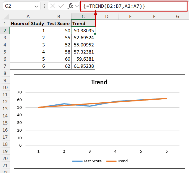
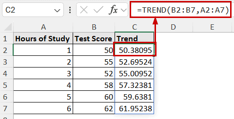
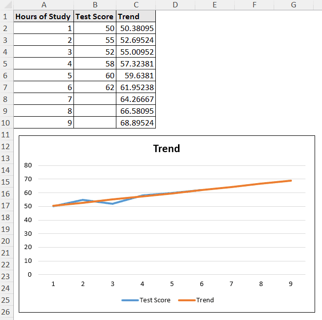
➤ Use the following formula in the output cell (C2) to find the linear trend values.
=TREND(B2:B7,A2:A7)
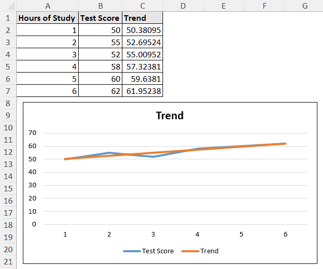
➤ Plot the new trend values and old y-values in a line chart by selecting these ranges and Insert >> Charts (group) >> Line.
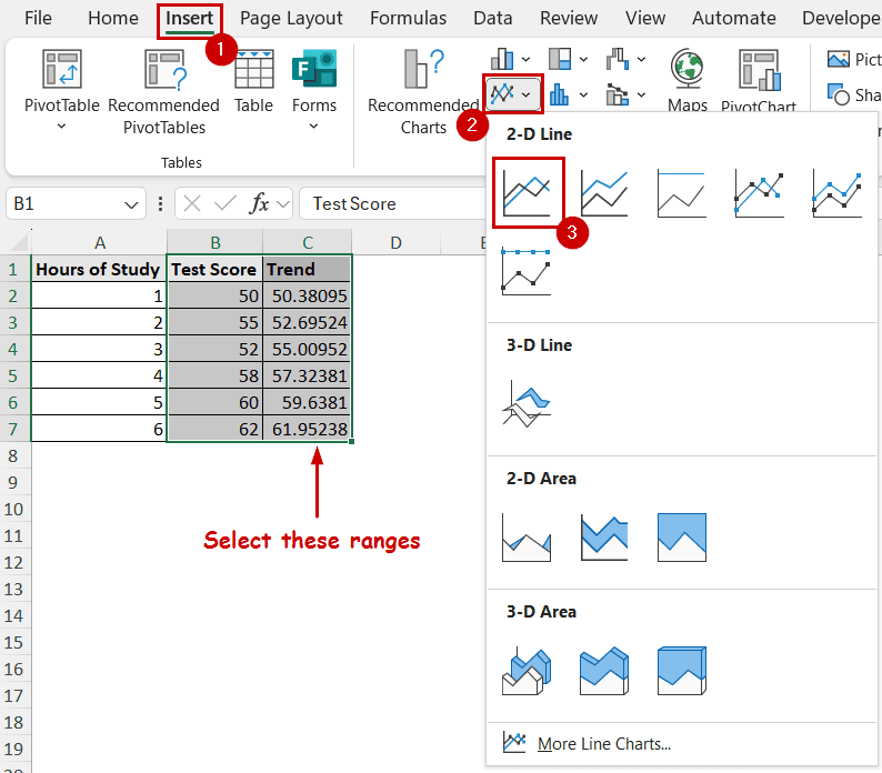
The trendline will be available in the chart.
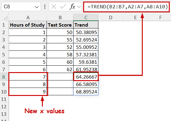
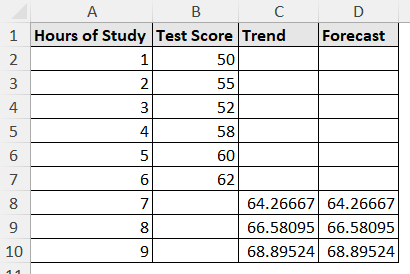
➤ To forecast other values, put them in a separate range (A8:A10) and insert the following formula in the output cell (C8).
=TREND(B2:B7,A2:A7,A8:A10)
➤ Insert the new data in a new line chart to display them.
Using FORECAST Function
The FORECAST function can be used interchangeably with the TREND function. The difference is that the TREND function usually returns the trend values on existing x values, while the FORECAST function returns these values for non-existent, future values.
Steps:
➤ Select the output cell and insert the following formula.
=FORECAST(A8:A10,B2:B7,A2:A7)

Both the TREND and FORECAST functions return the same values for future x values.
FAQ
What is the difference between FORECAST and TREND in Excel?
Both the FORECAST and TREND functions have the same functionality. The difference is in their arguments and argument types.
The FORECAST function can take both a single and an array of non-existent x values. It always predicts the linear trend y values of a non-existent x value. The TREND function can return for the existing as well as non-existent (future) x values while taking an array as an argument.
Can I calculate a trend for non-linear data?
If the data is scattered around a single trend, the calculation is still as straightforward as all of the demonstrations.
However, the trend, by definition, follows a linear pattern. If the data has a non-linear trend, you either have to calculate it by plotting a straight trendline for charts, or the functions will calculate assuming a trendline anyway.
What does the R-squared value indicate?
The R-squared value is the coefficient of determination. It measures how well a trendline equation fits with the existing data. A value of 0 indicates no fit, and 1 indicates a perfect fit. While there are no agreed-upon thresholds for a good scale, the closer it is to 1, the better.
Conclusion
By calculating trend analysis, we can forecast or predict future values and make informed decisions. We have covered three major ways to calculate trend analysis in Excel. We have used the chart’s built-in trendline feature, TREND, and FORECAST functions to find the trend values.
Feel free to download the practice workbook and give us your feedback.