Filtering data is not an uncommon practice for data analysis. While Excel already includes a handful of options for filtering, we sometimes need to filter our dataset with custom fields as well. In this article, we will learn how to filter a pivot table with a custom list.
➤ Add a helper column to the source table with the custom list.
➤ Refresh the pivot table.
➤ Add the new field to the pivot table.
➤ Drag the field to the Filters area
That was a long process, and it might have been difficult to follow due to the short explanation. Up next, we will be explaining how to do it in detail. Therefore, consider reading the full tutorial to learn the methods better.
Filtering a Pivot Table with a Custom List
We have a list of student grades in our spreadsheet here. Later, the authority asked to filter the table with the locations of the students. We have to integrate the list of cities as a custom list to filter the pivot table. Here is the process to do that:

Step 1: Adding the Custom List to the Existing Table
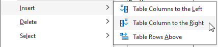
First, we need to add the “City” column to the existing table. The list cannot be directly integrated into the pivot table, adding it to the source table is the only way.
➤ Right-click on a cell of the rightmost column of the table, and go to Insert > Table Column to the Right
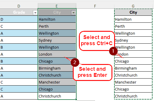
➤ Then, we copy the custom list and paste it into the new column. To do that, we select the custom list using the mouse and press Ctrl+C. Then we go to the new column, select all the rows, and press Enter. The whole list should be included in the table now.
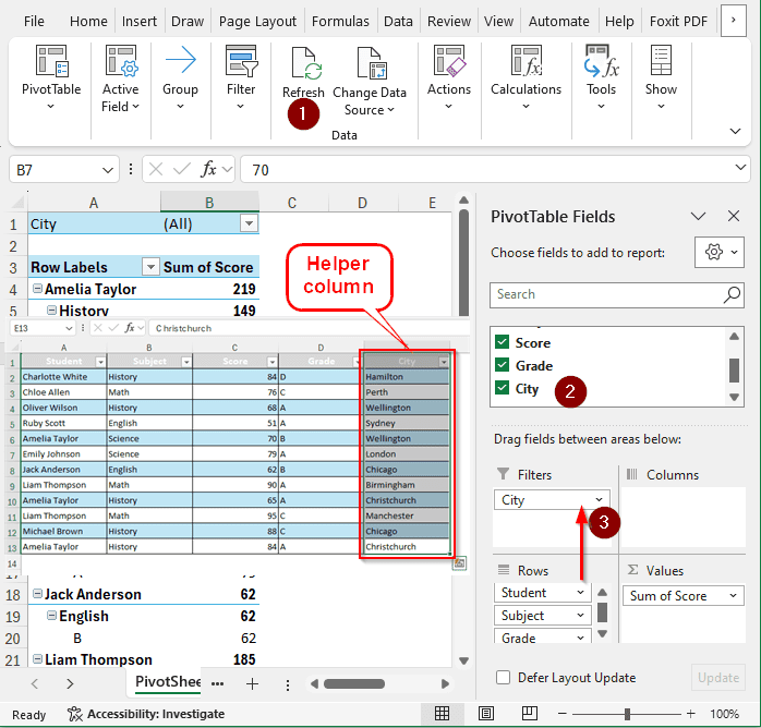
Step 2: Refresh the Pivot Table
The pivot table is not yet aware of the change in the source table. We need to make it aware of that.
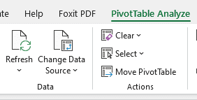
➤ After selecting a cell from the pivot table, we go to the “PivotTable Analyze” tab and click Refresh.
➤ From the “PivotTable Fields” panel, we check the “City” box. The box would now be available in the Rows area.

Step 3: Put the Filter in the Work
The new field is available now for use as a filter. Let’s make it work for our dataset.
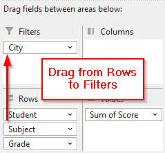
➤ Drag the “City” field to the “Filters” area.
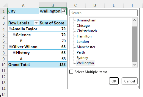
➤ Now we can filter using different cities, which is our custom list. You can also use multiple cities by checking the “Select Multiple Items” box.
Frequently Asked Questions
How do I filter a dynamic list in Excel?
The pivot table can automatically filter a dynamic list in Excel. However, if you don’t want to use a pivot table, there are functions to do the filtering. Write this formula to do so:
=FILTER(A1:A10, B1:B10 > 10)
Here, the A1:A10 is the range, and the condition is that if the data in B1:B10 is greater than 10, the values will be returned by the formula.
Can you filter in Excel based on a list?
After selecting your data set, you can go to the Data tab and choose Filter to create a filter. From the column header, open the arrow by clicking, and you will see the list of data in the column. You can filter out the rows you don’t want to see.
How do I add a slicer in Excel?
While you have the pivot table selected, go to the Insert tab. From the Filters section, select Slicer. From the Insert Slicer dialog box, you can choose the columns you want to filter using the slicer.
Can we apply filter in PivotTable?
Yes. To do so, go to the PivotTable Fields panel on the right and drag the rows/columns to the Filters area to make them a filter for the table. Now, you can apply the desired filter from the table directly.
How do I edit a pivot table?
You can edit the text fields in a pivot table directly from the table. However, the fields with numbers won’t be editable as Excel has to work with the values. For both of the fields, it is better to edit the source table rather than the pivot table.
How do I sort a table using a custom list?
Select the whole dataset of the table that you want to sort. From the Home tab, go to the Editing section, and click Sort & Filter > Custom Sort. A new pop-up will open. Select Custom List from the Order column. Then, in the new window, write the custom list and add it. Set Sort by to your desired column and click OK.
Wrapping Up
In this article, we have learned how to filter a pivot table with a custom list in Excel. The workbook we used for the tutorial is available for download. Make sure to practice on that spreadsheet before applying the methods to your own work. Leave a suggestion at the bottom, and we will see you in another Excel guide.