Often, we work with business or academic data spread across multiple worksheets and need to find certain information from these datasets. However, most of the time, using basic lookup formulas is time-consuming and leads to mistakes. Thus, we use the INDEX and MATCH functions to deal with such situations.
For example, you’re working with a dataset of residents where one sheet contains their demographic details, another contains employment status, and a third sheet lists their hobbies. Now, if you want to see a resident’s occupation or hobby using their name or phone number, doing it manually across sheets can be messy and time-consuming. Instead, if you use the INDEX and MATCH functions, you can pull the right information automatically and accurately.
In this article, we will explain how to use INDEX MATCH across multiple sheets in Excel to retrieve information.
➤ First, make a new sheet and rename it.
➤ Then make a drop-down table. Select cell A1 and write Information Table.
➤ Now, click on cell A2, and type Name.
➤ Then, select cell B2, and create a drop-down list by selecting Data from the upper menu bar. Then, go to Data Tools and select Data Validation.
➤ A new window will appear. Go to Settings> Validation Criteria> Allow, and choose List from the validation options.
➤ Now, in the box under Source, write down =Demographic-Info!A2:A6. Here, make sure you write the source sheet name exactly and also check the cell range twice to ensure it is right.
➤ Finally, select Okay, and you will see the drop-down icon in cell B2.
➤ Now, select cell A4 and write City.
➤ Then, click on cell B4 and insert the following formula:
=INDEX(‘Demographic-info’!C2:C6, MATCH(B2, ‘Demographic-info’!A2:A6, 0))
➤ Now, click on cell A5 and write Age.
➤ Then, select cell B5 and insert the following formula:
=INDEX(‘Demographic-info’!B2:B6, MATCH(B2, ‘Demographic-info’!A2:A6, 0))
➤ Now, select cell A6 and write Employment Position.
➤ Then, click on cell B6 and insert the following formula:
=INDEX(‘Employement-Status’!B2:B6, MATCH(B2, ‘Employement-Status’!A2:A6, 0))
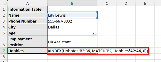
➤ Now, click on cell A7 and write down Hobbies.
➤ Then, select cell B7 and insert the following formula:
=INDEX(Hobbies!B2:B6, MATCH(B2, Hobbies!A2:A6, 0))
Steps to Use INDEX-MATCH Formula to Retrieve Data Across Multiple Sheets in Excel
The combination of the INDEX MATCH functions in Excel is a powerful tool to look up and retrieve data efficiently. When you work with multiple sheets, it allows you to find specific information from different sheets based on your given criteria.
To retrieve data across multiple sheets using INDEX MATCH, we will use specific sheet names inside our formula. This helps us to pull data from the desired sheet without rewriting formulas for each sheet manually.
We will use the following dataset to explain how to apply the INDEX MATCH functions to find information across multiple sheets in Excel. This dataset has three sheets containing a few residents’ Demographic information, Employment status, and Hobbies.
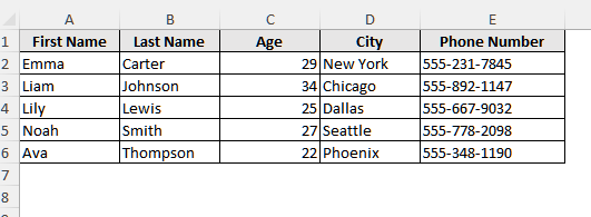
Sheet 1: Demographic Information
This sheet contains the resident’s name, age, phone number, and the city they are living in.
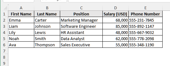
Sheet 2: Employment Information
In this sheet, we have additionally stored the residents’ salary and their respective positions in their organization.
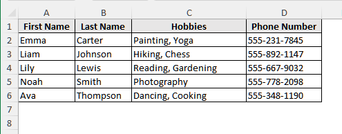
Sheet 3: Residents’ Hobbies
The final sheet is to keep a record of the resident’s hobbies and interests.
Now, we will create a drop-down table on a new sheet. In that table, if we select the name, we can automatically find their phone number, living city, age, occupation, and hobbies.
Step 1: Create the Sheet
To create a table to find relevant information across these three sheets, you need to first create a new sheet.
Steps:
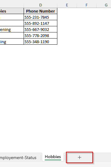
➤ First, click on the + (plus sign) at the bottom beside the last sheet name. It will open up a new sheet.
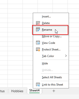
➤ Now, keep the cursor on the name of the new sheet and press the right button of your mouse. Then choose the Rename option and write any relevant name.
Step 2: Set Up the Look Up Fields
Now, we will set up a drop-down field for the resident’s name to find the relevant information about that person.
Steps:
➤ Select cell A1 and write Information Table.
➤ Now, click on cell A2, and type Name.
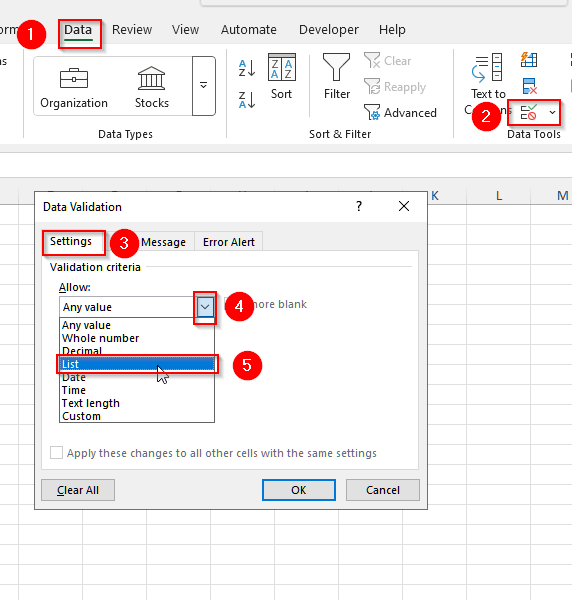
➤ Then, select cell B2, and create a drop-down list. To create it, first select Data from the upper menu bar. It will open up some new options. From these options, go to Data Tools and select Data Validation.
➤ Now, a new window will open up. Under the Setting option, you will see Validation Criteria. Then, click on the drop-down option under Allow bar. A new list of options will open up.
➤ Select List from the new options.
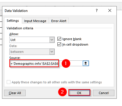
➤ Now, in the box under Source, write down =Demographic-Info!A2:A6. Here, make sure you write the source sheet name exactly and also check the cell range twice to ensure it is right.
➤ Finally, select Okay, and you will see the drop-down icon in cell B2.
Step 3: Set Up the INDEX MATCH Formula to Find Relevant Information
Now, we will use the INDEX MATCH functions to find different information about the residents from different sheets.
Steps:
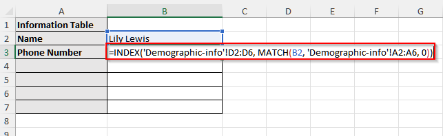
➤ Select cell A3 and write Phone Number.
➤ Then, click on cell B3 and insert the following formula:
=INDEX('Demographic-info'!D2:D6, MATCH(B2, 'Demographic-info'!A2:A6, 0))
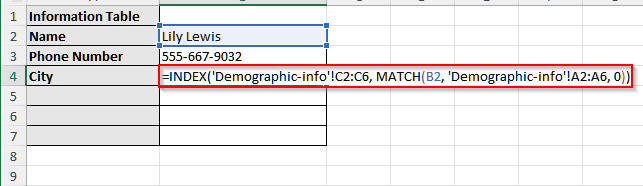
➤ Now, select cell A4 and write City.
➤ Then, click on cell B4 and insert the following formula:
=INDEX('Demographic-info'!C2:C6, MATCH(B2, 'Demographic-info'!A2:A6, 0))
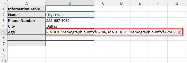
➤ Now, click on cell A5 and write Age.
➤ Then, select cell B5 and insert the following formula:
=INDEX('Demographic-info'!B2:B6, MATCH(B2, 'Demographic-info'!A2:A6, 0))
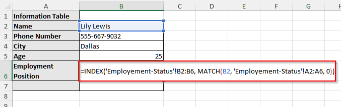
➤ Now, select cell A6 and write Employment Position.
➤ Then, click on cell B6 and insert the following formula:
=INDEX('Employement-Status'!B2:B6, MATCH(B2, 'Employement-Status'!A2:A6, 0))
➤ Now, click on cell A7 and write down Hobbies.
➤ Then, select cell B7 and insert the following formula:
=INDEX(Hobbies!B2:B6, MATCH(B2, Hobbies!A2:A6, 0))
➤ Finally, the dropdown table to find some relevant information about the residents using INDEX MATCH functions is completed. Now, if you change the Name, all the other related information in the table will also change.
➥ Here, the first part, array, means the range of the value the function will return. Such as our phone number was cell D2 to D6 in the Demographic-info sheet, and so, in the formula to find the phone number, our array was 'Demographic-info'!D2:D6.
➥ In the second part, we will write our lookup array inside the Match function. In our formula for finding the phone number, this part was MATCH(B2, 'Demographic-info'!A2:A6, 0).
➥ Here, B2 cell refers to the cell where our lookup value is. In our data, B2 cells contain the drop-down list of names.
➥ Then, comes our lookup array, 'Demographic-info'!A2:A6. This is the cell range where Excel will match the lookup value and then return the result.
➥ Finally, the last attribute 0 represents an exact match.
Frequently Asked Questions
Why Is My INDEX MATCH Returning Zero?
If your INDEX MATCH formula returns 0, it may be because the matched cell is empty, or the return column is misformatted as a number instead of text. Suppose your data is in cells B2 to B7, but in the formula, you wrote D2 to D7 for the first array, while D2 to D7 are just empty cells. Then the INDEX MATCH formula will return 0 (Zero)
Why Is My Excel Freezing After Using Index Match?
If your INDEX MATCH formula references a very large range, your Excel might freeze after using it. Because finding and matching in a large range can slow down performance, especially on older computers or large workbooks. To fix this, limit the lookup ranges to smaller, specific ranges (like A2:A100 instead of A: A).
Wrapping Up
In this article, we learned to use the INDEX MATCH function to find information from multiple sheets in Excel. These functions give us accurate results and save us time. Try these functions to fetch important information from your multi-sheet Excel dataset and share your thoughts with us.

