Want to emphasize recent data points while smoothing out noise in your Excel charts? That’s exactly what a weighted moving average is for. Instead of treating every value equally like a simple average, this method gives more importance to newer or more relevant entries. It’s incredibly useful for forecasting sales, stock prices, or any time-based trend where the latest numbers matter most.
In this article, you’ll learn multiple ways to calculate a weighted moving average in Excel, including formulas using SUMPRODUCT and dynamic weighting with helper columns. Each method comes with step-by-step instructions and sample data so you can implement them right away.
Steps to calculate weighted moving average in Excel:
➤ Create a new column next to your data.
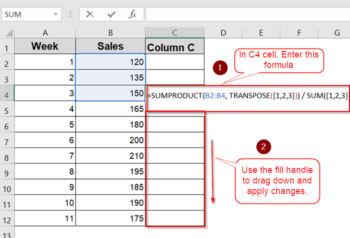
➤ Insert formula: =SUMPRODUCT(B2:B4, TRANSPOSE({1,2,3})) / SUM({1,2,3})
➤ Press Enter.
➤ Drag down to the rest of the cells.
Weighted Moving Average in Excel: What It Means & How It Works?
When someone searches for “weighted moving average in Excel,” they’re typically looking to analyze data trends using a method that gives more importance to recent values. A weighted moving average (WMA) is a type of moving average where each data point is multiplied by a predefined weight before calculating the average. This is particularly useful in financial forecasting, sales tracking, or any scenario where recent values should influence the result more than older ones.
Use Manual Weighing with SUMPRODUCT and SUM
This method is ideal for small-to-medium datasets where you define the weights manually. It provides full control over the calculation and is easy to apply if you want to highlight recent values more heavily.
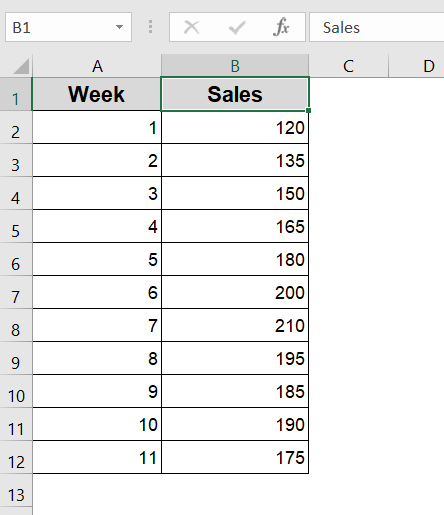
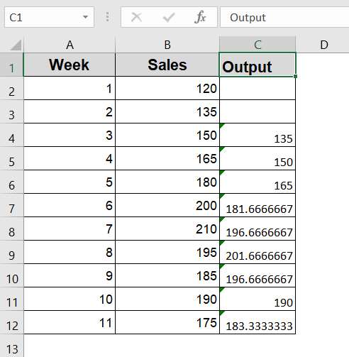
We’ll use a basic dataset showing weekly sales figures. Our goal is to calculate the weighted moving average over a 3-week period, giving more importance to the latest week.
Steps:
➤ Decide on your weights. For example, to emphasize recent data: 3 (most recent), 2, and 1
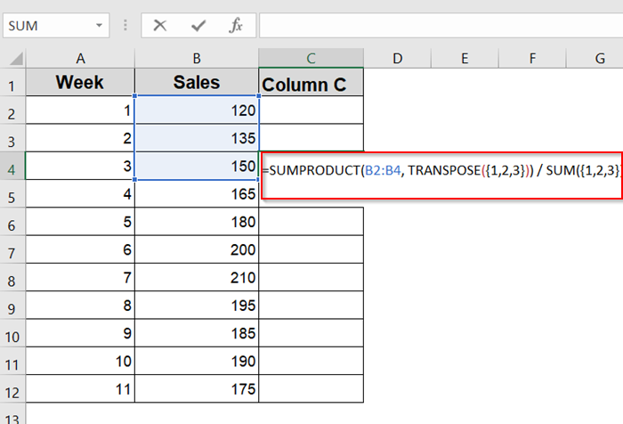
➤ In a new column (say Column C), enter this formula starting from cell C4:
=SUMPRODUCT(B2:B4, TRANSPOSE({1,2,3})) / SUM({1,2,3})
➤ Drag the formula down from C4 to C12 to apply it to the rest of your data.
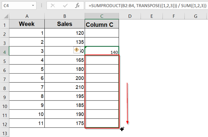
➤ Each cell will now show a weighted moving average of the current and two previous sales figures.
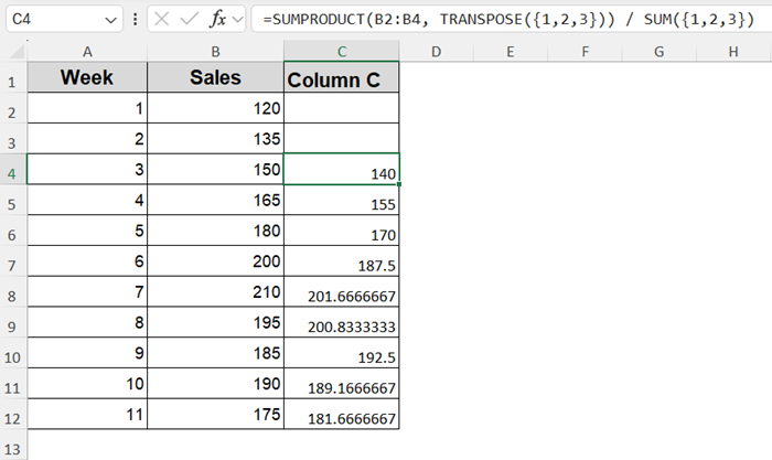
This setup gives more emphasis to recent sales data which is perfect for trend forecasting.
Use Helper Columns for Custom Weighting
This approach is useful when your weights may change often or are stored alongside your data. By using helper columns, you make the sheet easier to update without rewriting formulas.
We’ll assign custom weights in a new column and use SUMPRODUCT to apply those dynamically.
Steps:
➤ Add a “Weights” column next to your data (e.g., Column C)
➤ In column D (starting from D4), use:
=SUMPRODUCT(B2:B4, C2:C4) / SUM(C2:C4)
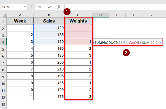
➤ Drag the formula down. Adjust the ranges (e.g., B2:B4 and C2:C4 for D4) as needed to align weights with the sales data.
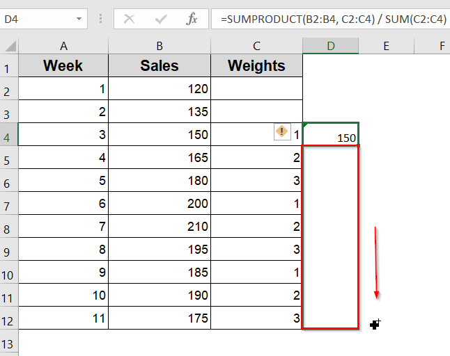
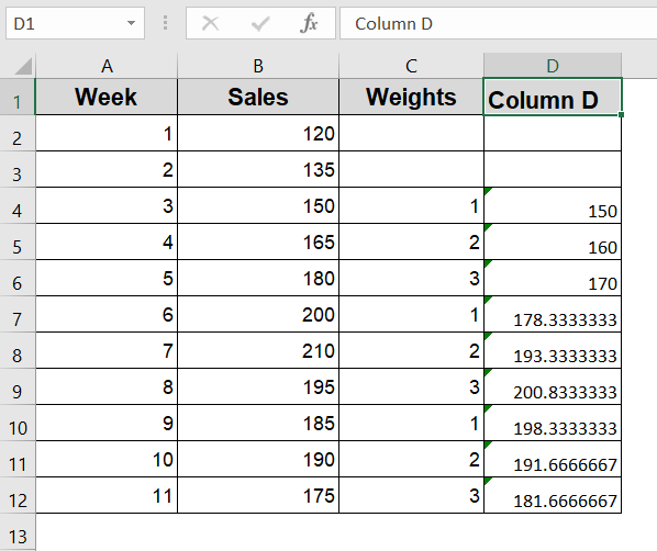
Now you can change any weight in Column C and the results in Column D will update automatically.
Use Data Analysis Toolpak (for Simple Moving Average Only)
While not built for weighted moving averages, the Analysis Toolpak is useful for quick simple moving averages. It’s a built-in feature and gives a fast visual overview of data smoothing.
This method doesn’t apply weighting but can be used as a reference point before applying custom logic like WMA.
Steps:
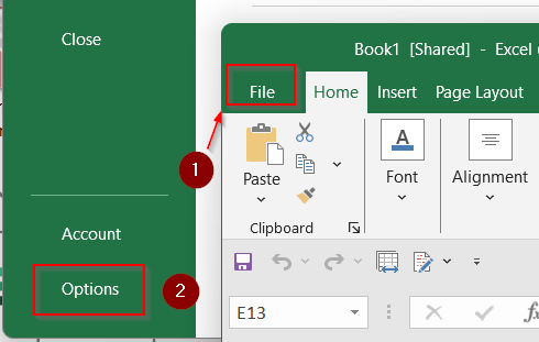
➤ Go to File >> Options.
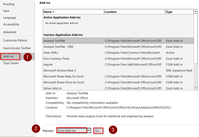
➤ Go to Add-ins. Under Manage, select Excel Add-ins and click Go.
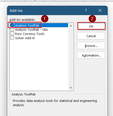
➤ Check Analysis ToolPak and click OK.
➤ Go to Data >> Data Analysis >> Moving Average.
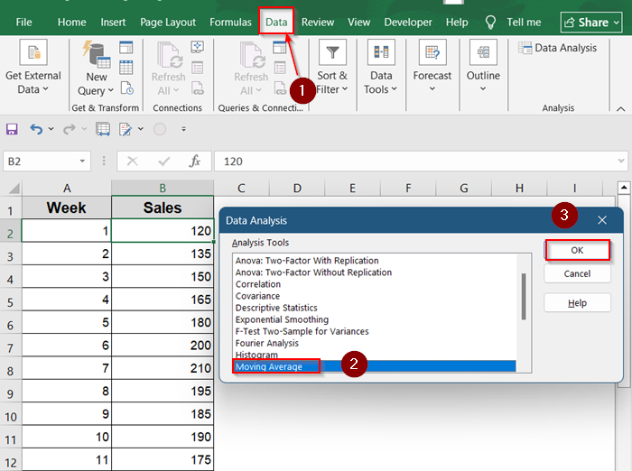
➤ Select your Sales range, set the Interval to 3, and choose where to place the output.
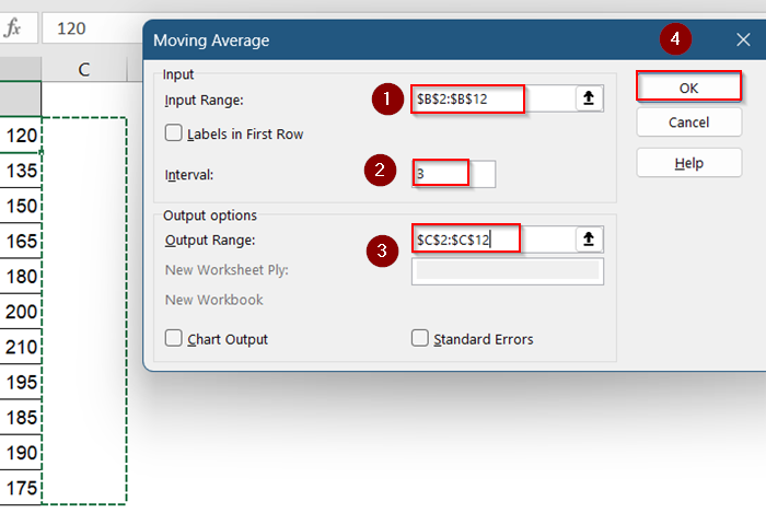
This provides a simple moving average. To mimic a weighted version, you’ll need manual formulas as shown above.
Frequently Asked Questions
How is a weighted moving average different from a simple moving average in Excel?
A weighted moving average gives more importance to recent data by applying different weights, while a simple moving average treats all values equally. WMA offers better trend sensitivity.
Can I use built-in Excel functions for weighted moving average?
Excel doesn’t have a dedicated WMA function, but you can use SUMPRODUCT with SUM to calculate it efficiently. This combo lets you define weights manually or dynamically.
What if I want a 5-point weighted moving average instead of 3?
Simply adjust your formula ranges and weights accordingly. For a 5-point WMA, change the cell ranges from B1:B3 to B1:B5 and update the weights array to {1,2,3,4,5}.
Does the weighted average work with dates and text in Excel?
WMA only works on numeric data. Dates and text can be included in your table but cannot be part of the actual averaging formula unless converted to numbers.
Is there a way to automate weight changes in Excel?
Yes, you can use a separate column or named range to store weights and reference them in your SUMPRODUCT formula. This allows you to update weights without editing formulas manually.
Wrapping Up
In this tutorial, we learned how to calculate a weighted moving average in Excel using manual formulas, helper columns, and simple averages with the Toolpak. Each method suits different levels of complexity, from basic 3-point WMA to advanced weight optimization. Feel free to download the practice file and share your thoughts and suggestions.