How to Add Axis Titles in Excel (2 Quick Methods)

Axis titles are labels that appear alongside the horizontal or vertical axis.

Axis titles provide context on what the axes represent. They provide more clarity to the chart, which is the point of creating charts in the first place.

You can add axis titles in Excel in two ways: using the Chart Elements button and the Chart Design tab.

In this tutorial, we will explore how to add axis titles in Excel.

The Chart Element button and the Chart Design tab are both relatively newer features in Excel. You will find the Layout tab instead of Chart Design in the older versions. You can use that tab instead and follow the second method in those Excel versions.

The “Chart Element” is one of the buttons that appears on the top-right of a chart after selecting it.

It is the + icon. The feature was introduced in Excel 2013. It’s purpose is to quickly add or remove different elements of the chart.

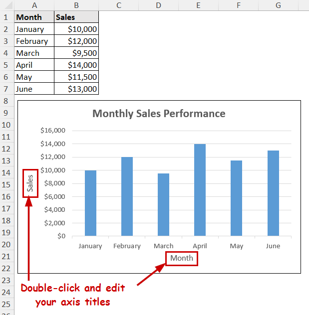
The following image shows a set of data tracking sales over different months.

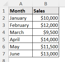
We have created a column chart based on the data.

We are going to add axis titles using the chart elements tab in the following steps.

Steps:

➤ Select the chart by clicking on it.
➤ Click on the Chart Elements button.
➤ Check the Axis Titles option.

➤ You can also click on the right arrow beside the Axis title option and select the horizontal or vertical axis title option individually.

➤ Double-click on the titles that appear after that. Then insert your title.

This is the most straightforward process to add axis titles in a chart in Excel.

Two new tabs appear on the ribbon after selecting a chart: Chart Design and Format.

You can add different chart elements from the Chart Design tab. That includes axis titles.

Steps:

➤ Select the chart.
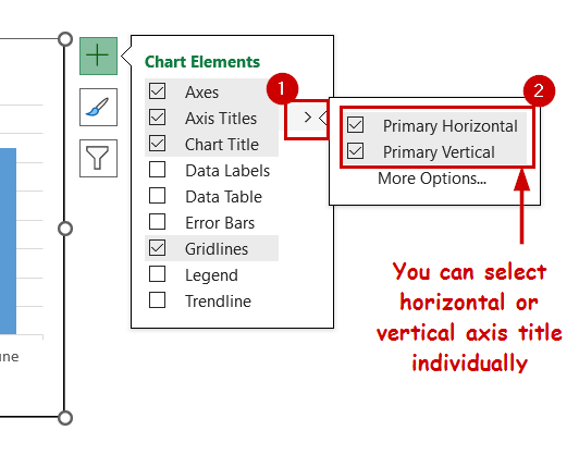
➤ Go to Chart Design >> Chart Layouts (group) >> Add Chart Element.
➤ Then select Axis Titles from the dropdown.
➤ Select Primary Horizontal, Primary Vertical, or both, depending on your preference.

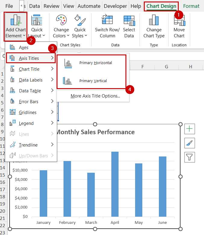
➤ Double-click on the axis titles and rename them after that.

FAQ

How do I remove axis titles in Excel?

You can remove axis titles by unchecking them from the Chart Elements button’s options. If you are using the Chart Design tab, selecting the axis titles option again will remove them.

There is another way to remove any chart element: selecting and pressing the  Delete  button on the keyboard. You can remove any axis title this way too.

Can I add axis titles to all chart types in Excel?

You can only add axis titles if the chart type has an axis. Charts like pies or doughnuts don’t have any axis. Thus, you can’t add axis titles to those types of charts.

How do I add a secondary axis title in Excel?

To add a secondary axis title, you need to have a secondary axis first.

You can add a secondary axis from a suitable data source (with more than two columns of data). After creating the chart, double-click on any series and select Secondary Axis from the Format Data Series pane.

Now, follow any of the processes in the methods above. You can find additional options for secondary axis titles.

Wrapping Up

In this tutorial, we have discussed how to add axis titles in Excel.

We have covered how to add axis titles from the Chart Elements button and the Chart Design tab.

In the older versions, you can find the “Layout” tab instead of Chart Design, where you will find the same options and follow the same procedure.

Feel free to download the practice file and let us know about your feedback.