Bar charts are a great way to compare different categories in Excel, and sorting the bars from largest to smallest makes it easier to see the top values right away. But Excel doesn’t have a direct option to sort a bar chart by itself. Instead, the order of the bars depends on how the data is arranged in your worksheet. So, if you want the bars to show in descending order, you need to sort or adjust the source data first. Whether your data is small or changes often, there are a few ways you can do this to make your chart show the bars in the order you want.
In this article, you’ll learn different ways to sort your data and make your bar chart display in descending order. We’ll explore methods like using Excel’s built-in Sort tool, applying formulas for dynamic sorting, adding helper columns, and adjusting the chart axis to get the order customized.
Steps to sort a bar chart in descending order in Excel:
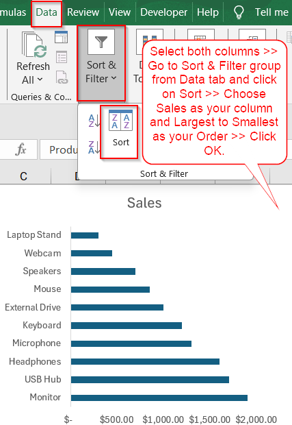
➤ Select the entire dataset including both columns (Product and Sales).
➤ Go to the Data tab on the Ribbon.
➤ Click Sort in the “Sort & Filter” group.
➤ In the Sort dialog box, under Column, select the “Sales” column.
➤ For Sort On, keep “Values” selected.
➤ For Order, select Largest to Smallest.
➤ Click OK.
Sort Data Using Excel’s Built-in Sort Tool
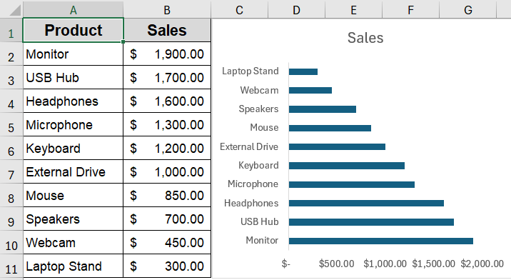
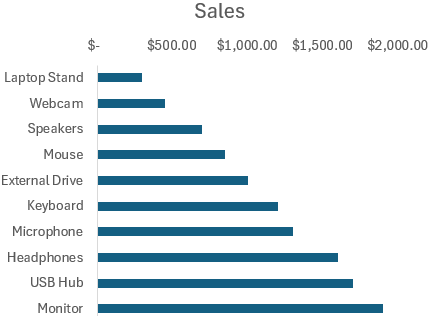
The simplest way to sort a bar chart in descending order is by sorting the underlying data using Excel’s Sort tool. When you sort the sales figures in the sample dataset from largest to smallest, the products will rearrange so that the highest-selling items appear first. This directly affects the bar chart linked to this data, updating it to display bars from longest to shortest, making it easy to see which products lead in sales.
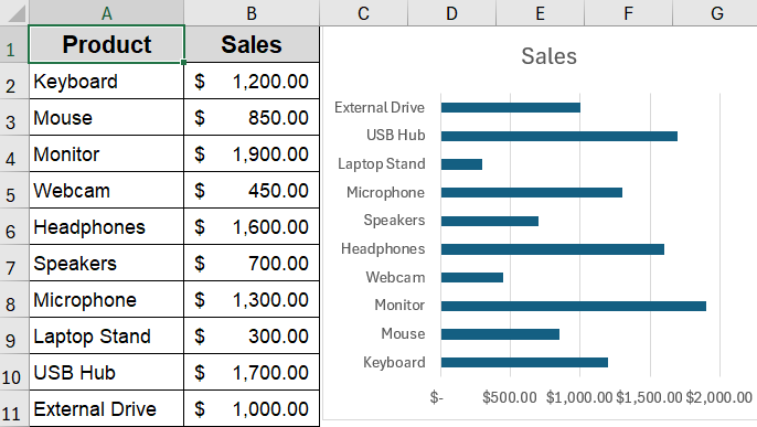
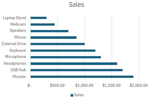
Here’s a sample dataset with 10 products and their sales figures to try out the sorting methods and see how the bar chart updates accordingly.
Steps:
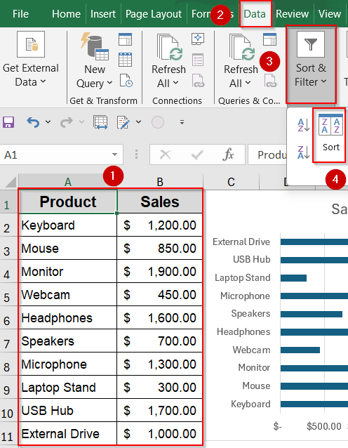
➤ Select the entire dataset including both columns (Product and Sales).
➤ Go to the Data tab on the Ribbon.
➤ Click Sort in the “Sort & Filter” group.
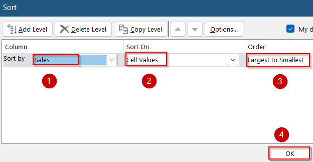
➤ In the Sort dialog box, under Column, select the “Sales” column.
➤ For Sort On, keep “Values” selected.
➤ For Order, select Largest to Smallest.
➤ Click OK.
Your data will be sorted in descending order, and if your bar chart references this range, it will automatically update to reflect the sorted order.
Apply the SORT Function for Dynamic Sorting
When you’re working with a dataset that updates frequently like monthly sales figures or live performance data, you might want your bar chart to stay in descending order automatically. Instead of sorting the data manually every time, you can use Excel’s SORT function to generate a live, sorted table that feeds directly into your chart. This approach ensures your visual stays accurate and always highlights the top-performing items first.
Steps:
➤ Next to your original data, create a dynamic sorted table using this formula in D2 cell:
=SORT(A2:B11, 2, -1)
Here, A2:B11 refers to your original dataset range, 2 tells Excel to sort based on the second column (Sales), and -1 specifies descending order.
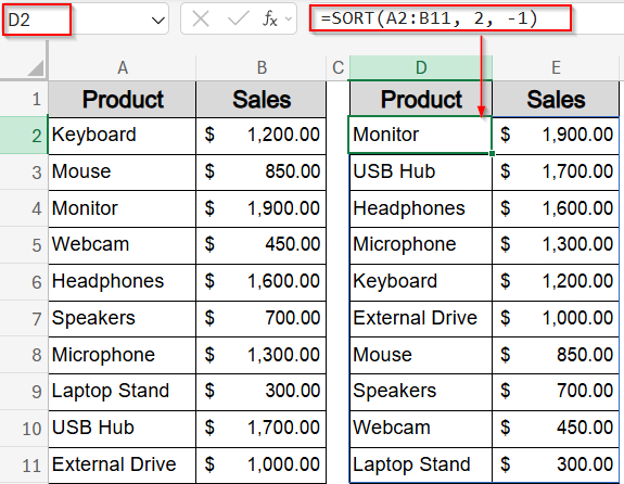
The formula will spill automatically creating a sorted table in descending order.
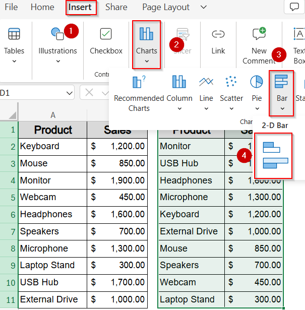
➤ Create your bar chart based on this sorted table instead of the original data by selecting D1:E11 and going to Insert tab >> Bar Chart.
Now, whenever your original data changes, your sorted data and chart update automatically.

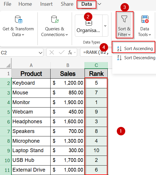
Use a Helper Column with RANK Function
If you want your bar chart sorted in descending order without altering the original sequence of your dataset, using a helper column with the RANK function is a smart workaround. This method lets you rank each value and then sort the data by rank, all while keeping your original product order intact for reference.
Steps:
➤ Add a helper column named “Rank” next to your Sales data.
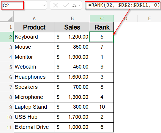
➤ In cell C2 (assuming data starts from row 2), enter:
=RANK(B2, $B$2:$B$11, 0)
This ranks the sales value in B2 compared to the entire range from B2 to B11, with 0 indicating descending order (highest value gets rank 1).
➤ Drag the formula down to C11.
➤ Sort your entire dataset by this “Rank” column in ascending order (smallest to largest).
Your bar chart linked to this sorted data will now show bars in descending order.
Sort Categories Using Axis Options by Reversing Order
If you’ve already inserted a bar chart and don’t want to modify the original data, Excel lets you flip the order of the bars directly from the chart settings. This method doesn’t actually sort your dataset, it simply changes how the categories are displayed on the vertical axis. By reversing the axis, you can visually arrange the bars from largest to smallest, making your chart appear in descending order without touching the cells underneath.
Steps:
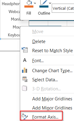
➤ Click on the vertical axis (category axis) of your bar chart.
➤ Right-click and select Format Axis.
➤ In the Axis Options pane, check the box Categories in reverse order.
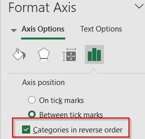
➤ This will flip the category order on the axis, effectively sorting the bars in descending order visually.
Note:
This method only reverses the existing order and requires your data to be sorted ascending first or prepared accordingly.
Insert a Pivot Table to Sort a Bar Chart in Reverse Order
Using a Pivot Table is an effective way to organize and sort large datasets quickly, especially when you want your bar chart to update dynamically with easy sorting options. By creating a Pivot Table from your data and sorting it within the Pivot Table itself, you can build a bar chart that reflects this sorted order automatically, without manually rearranging your original data.
Steps:
➤ Select your entire dataset, including both the category and value columns.
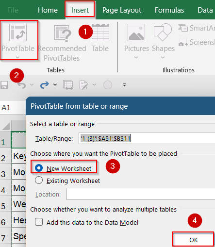
➤ Go to the Insert tab on the Ribbon and click PivotTable.
➤ In the Create PivotTable window, choose where to place the Pivot Table (new or existing worksheet) and click OK.
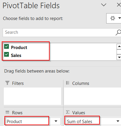
➤ In the PivotTable Fields pane, drag the category field (e.g., Product) to the Rows area.
➤ Drag the value field (e.g., Sales) to the Values area.
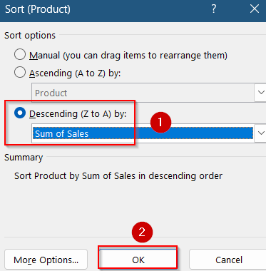
➤ Click the drop-down arrow next to the Row Labels in the Pivot Table, select Sort, then choose More Sort Options.
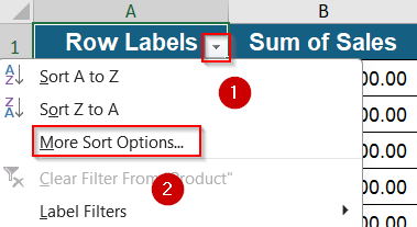
➤ Select Descending (Z to A) by Sum of Sales (or your value field) and click OK.
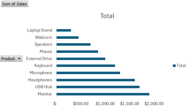
➤ Now, create a bar chart based on the Pivot Table data by going to Insert tab >> Bar Chart.
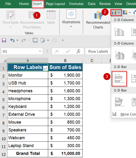
Your bar chart will automatically display the categories sorted from highest to lowest value, and any updates to the original data will be reflected when the Pivot Table is refreshed.
Frequently Asked Questions
Can I sort a bar chart directly without changing the data?
Excel doesn’t offer a direct way to sort a bar chart visually. The order of bars always depends on how the source data is arranged, so any sorting must happen at the data level or by reversing the axis.
What if my chart doesn’t update after sorting the data?
If your bar chart doesn’t reflect changes after sorting, double-check the data range it’s linked to. Charts built from static or non-contiguous selections may not respond to sorting unless you update the source range manually.
Does the SORT function work in all versions of Excel?
No, the SORT function is only available in newer versions like Excel 365 and Excel 2021. If you’re using Excel 2019 or earlier, you’ll need to sort manually or use helper columns with formulas like RANK.
Will reversing the axis change my actual data order?
Reversing the category axis only changes how your chart looks. However, it doesn’t affect the order of the data in your worksheet. It’s purely a formatting option that flips the bar direction for better visual clarity.
Which method should I use for charts that update frequently?
For dynamic datasets that change often, the best approach is using the SORT function. It keeps your sorted table and chart updated automatically, so you don’t have to re-sort manually every time data is added or changed.
Wrapping Up
In this tutorial, we learned multiple ways to sort a Bar Chart in descending order in Excel from basic manual sorting using built-in tools like Sort to more dynamic solutions using functions such as RANK and SORT. Whether you’re working with static data or live reports, these methods help ensure your charts always highlight top values clearly. Feel free to download the practice file and share your feedback.