Error bars are horizontal or vertical lines in data points that show the confidence level of the data in the sample. Custom error bars in Excel represent different variability for different data points.
An error bar shows the uncertainty of the data with reference to the sample size. It indicates data variability of the sample and can be used to compare variability between series.
To add custom error bars in Excel,
➤ Select a chart.
➤ Go to Chart Elements >> Error Bars >> More Options.
➤ Select Custom in the Format Error Bars pane and click on Specify Value.
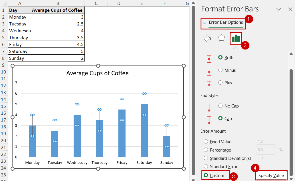
➤ Select proper values for the positive and negative fields in the Custom Error Bars dialog box.
In this tutorial, we will demonstrate how to add custom error bars in Excel. The main way to add custom error bars is through the Format Error Bars pane. Whether we choose the Chart Elements button or the Chart Design tab, the main goal is to access the Format Error Bars pane. Then use the options available there to add or customize error bars.
Download Practice WorkbookQuick Video Tutorial: Add Custom Error Bars in Excel
Add Custom Error Bars Using the Chart Elements Button
The Chart Element button is the plus icon that appears at the top-right after selecting a chart in Excel.
The button gives quick access to add, modify, or remove different elements to the chart. We can add fixed value, percentage, or standard deviation error bars from the button directly.
To add more customizable error bars, we need to open the Format Error Bar pane using the button.
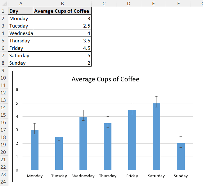
This is a column chart we are using for demonstration. The chart shows the average cup of coffee consumption throughout the week for a sample.
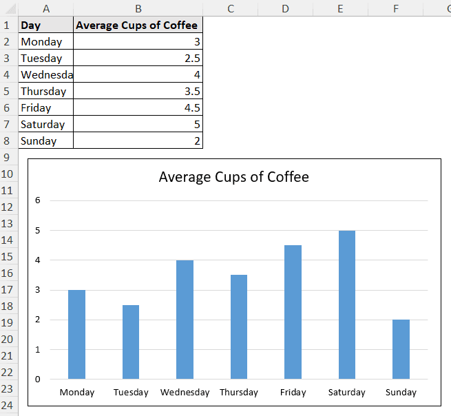
We are going to add a custom error value of 0.5 on the positive side and 0.3 on the negative side.
Steps:
➤ Select the chart.
➤ Go to Chart Elements >> Error Bars >> More Options.
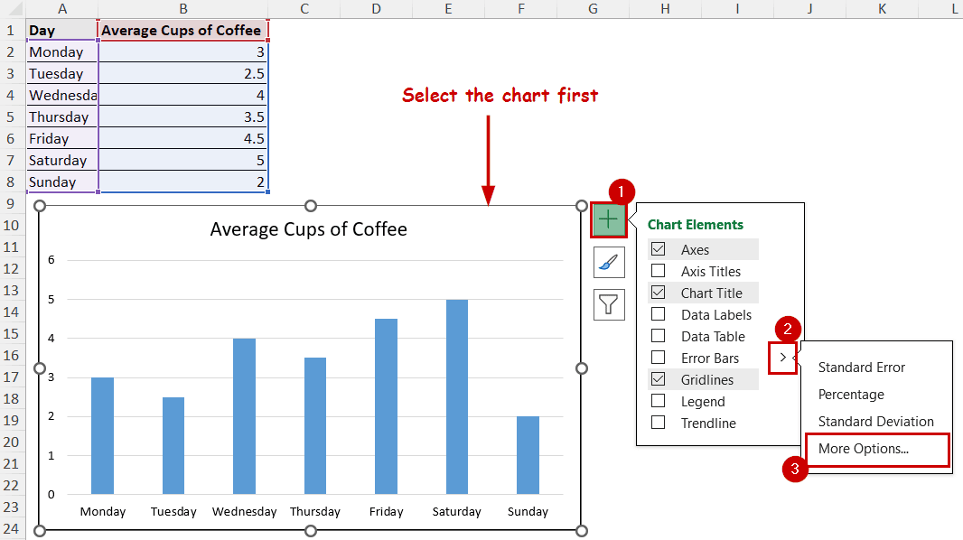
The Format Error Bars pane will open up.
➤ In the Format Error Bar pane, select the Error Bar Options. Then select Custom and click on the Specify Value button.
➤ Insert the proper values for the positive and negative value fields in the Custom Error Bars dialog box.
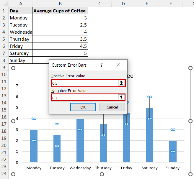
➤ Click on OK.
The error bars will now be set to a custom value.
Using Chart Design Tab
After selecting a chart, two new tabs open in the ribbon: Chart Design and Format.
The Chart Design tab offers the option to add different elements, including the error bars. Through this option, we can access the Format Error Bars pane too to customize the error bars.
Steps:
➤ Select the chart.
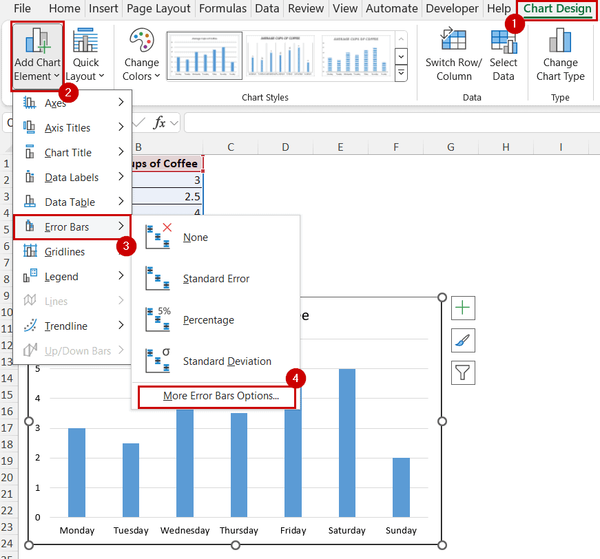
➤ Go to Chart Design >> Chart Layouts (group) >> Add Chart Element.
➤ Select Error Bars >> More Error Bars Options.
➤ In the Format Error Bars pane, select Custom. Then click on the Specify Value button.
➤ Select proper values in the fields of the Custom Error Bars dialog box.
➤ Click on OK.
The result will be the same as the previous one.
Note: The two methods use the same options. We are just accessing them differently.
FAQ
How to customize individual error bars in Excel?
To customize an individual error bar instead of all error bars, as shown in the methods, you need to select one specifically.
To select one error bar, click on an error bar first. It will select all the error bars. Then click on it again. Now, Excel will select the error bar you are clicking on. Now make the intended changes to the error bar.
How to add confidence interval error bars in Excel?
To add confidence interval error bars, use the (100-confidence interval) values for positive and negative values in the Custom Error Bars dialog box. You can use any of the methods from the article up to that point.
You can also have a marginal error for each series and insert the sheet reference in the Custom Error Bars dialog box.
How do I remove error bars from my chart?
To remove error bars, select the error bars and press Delete on your keyboard. You can also uncheck them from the Chart Elements button or the Chart Design tab.
Conclusion
In this article, we have covered the two ways to add custom error bars in Excel. We have demonstrated methods to use the Chart Element button and the Chart Design tab to open the Format Error pane. Then, we have used the pane to add custom error bars or customize already existing error bars.
Feel free to download the workbook and give us your feedback.