In personal finance or cash calculation, calculating the running balance is mandatory. In a store, you want to know how much liquid cash is in the drawer so that you can pay regular bills and expenses. In this tutorial, we will learn how to use the running balance formula in Excel based on different cases or criteria.
➤ In the column of running balance, write this formula in the first row (other than the heading):
=SUM($D$2:D2)
➤ Replace $D$2:D2 with the current balance cell, keep the first cell as an absolute reference.
➤ Autofill the entire column to get the full running balance.
That was a simple method for calculating the running balance. But there are even simpler methods to do so. Moreover, there can be cases where you have cash withdrawals and deposits, where this method won’t work. In this tutorial, we will show you all the methods to calculate running balance in Excel. Study and follow them to get a proper understanding of calculating the running total for yourself.
Basic Mathematical Sum to Calculate Running Balance
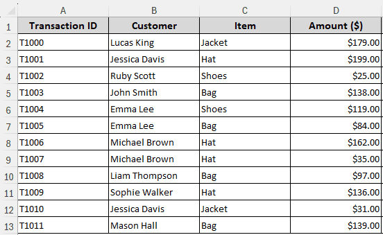
This is the simplest running balance formula you can use in Excel. We are going to use the plus (+) sign to sum up the balance and call it a day. To demonstrate, we have a dataset with some retail transactions. There are dollar amounts for each transaction, and we are going to calculate the running total from the table. Let’s begin:
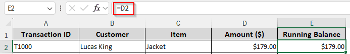
➤ We are using column E for calculating the running balance. In cell E2, write this formula:
=D2
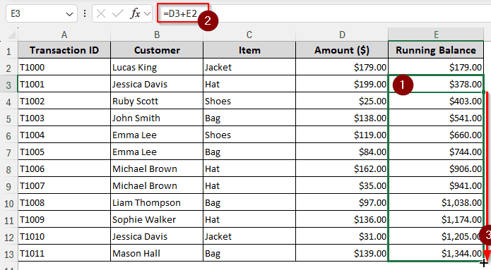
➤ In E3 cell, write this formula:
=D3+E2
➤ Autofill the entire column by dragging the plus (+) sign at the bottom-right corner of the E3 cell to get the running balance.
Making Use of the SUM Function
In the previous function, we used mathematical expressions to calculate the running balance. However, that required us to use two different formulas. If we want, we can use a single formula for the whole column. The SUM function in Excel takes a range (or a list of values) and sums it up. We will use this function for this method. Here is how to do that:
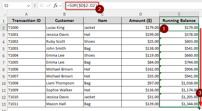
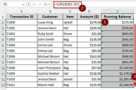
➤ In the helper column E, navigate to E2 cell, and write this formula:
=SUM($D$2:D2)
➤ Click and drag the plus (+) sign using your mouse cursor to complete the whole column.
Conditional Running Balance Using SUMIF
So far, the running balances we did were for a single account. But customers like multiple payment options. If they pay the amount in different banks, we might need to find the running balances of all those accounts.
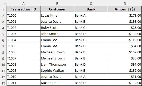
The SUMIF function is similar to the SUM function, but you can ask it to adhere to a condition. We have slightly modified the dataset to include multiple banks instead of the item names. Time to learn the steps to calculate the conditional running balance:
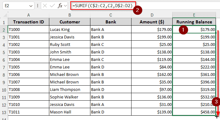
➤ In the column for running balance, write this formula in the desired cell, then autofill the whole column.
=SUMIF(C$2:C2,C2,D$2:D2)
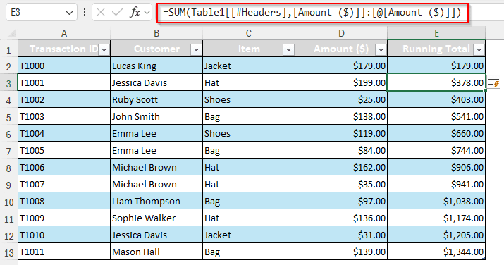
Running Balance in a Table
Calculating running balance in a table is different than normal calculation. Excel completes the table formulas in a distinctive way, and we have to adapt. Once we do, it actually works better than a regular range, as regular range calculation will have issues if you have to add or move a row.
➤ In the new column, write this
=SUM(
➤ Now, click on the row heading of the amount (D1 cell). This will refer to the whole column.
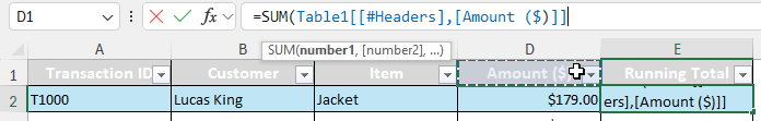
➤ Click on the formula (right after ]]) and give a colon (:). Then click on the D2 cell. This will make excel refer to the cell of the cash amount. Write ) to close the bracket and complete the formula.
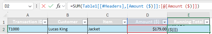
➤ Press Enter to complete the whole column. As it’s a table, excel will fill up the remaining rows, we don’t have to autofill by ourselves.
Conditional Running Balance in a Table Using SUMIF
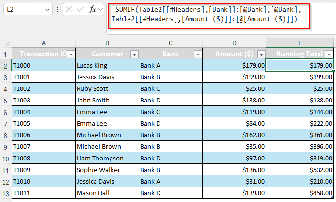
We are changing the formula for the conditional running balance to accommodate a table. The formula will be bigger, but it will work better. Here are the steps to calculate the running balance in a table with a condition.
➤ Write this formula in the helper column under the heading cell:
=SUMIF(Table2[[#Headers],[Bank]]:[@Bank],[@Bank],Table2[[#Headers],[Amount ($)]]:[@[Amount ($)]])
➤ Press Enter to fill the whole column.
Finding the Running Balance from Cash Inflows and Outflows
For all of the methods done before, we calculated the running total using cash inflows only. But in a realistic scenario, there will be inflows and outflows in retail stores. Even if you are doing this for your personal finances, chances are you are expending in most of the transactions. Therefore, we must learn how to calculate the running balance when we have both inflows and outflows.
To demonstrate this method, we have a dataset with deposits and withdrawals. We are going to calculate the running balance considering both of them at the same time. Follow the steps below:
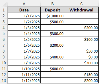
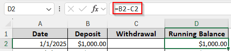
➤ Create another column for the Running Balance. We are choosing column D for this.
➤ In D2 cell, write this formula:
=B2-C2
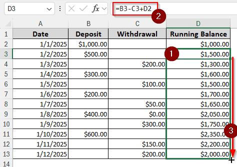
➤ In D3 cell, write this formula:
=B3-C3+D2
➤ Autofill the whole column to complete the calculation of the running balance.
Calculate Running Balance from Deposits and Withdrawals
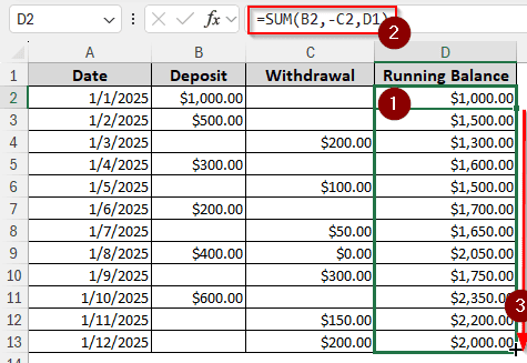
Instead of using mathematical signs like the previous method, we can use the SUM function to calculate the running balance. Like the last time we calculated using SUM, we still get the benefit of using the same formula for all of the rows. Here is how to make use of the formula:
➤ You know what to do already, write this formula in your target cell:
=SUM(B2,-C2,D1)
➤ Autofill the column to finish the calculation.
OFFSET with SUM to Calculate Running Balance from Inflows and Outflows
You might want to know why we need to mix OFFSET with SUM, as the latter already works for our job. There are actually a number of issues that can happen with SUM. The SUM function refers to the previous cell to calculate the current balance. So, if you remove a row, the function will not work anymore. If you insert a row, the formula is not updated, so the balance gives false output. Even worse, when you move a row, the cell reference might be messed up in a hard-to-detect way.
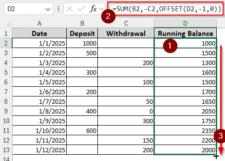
To resolve those issues, you need to use OFFSET to do the cell referencing part. The OFFSET function returns the reference of a cell depending on the cell where the function is used. Read the steps below to know how to do that:
➤ Use this formula to calculate the balance:
=SUM(B2,-C2,OFFSET(D2,-1,0))
➤ Autofill the column if you are in a data range. If you are using a table, only pressing ENTER is enough to fill the whole column.
Frequently Asked Questions
What is the formula for running balance in sheets?
It is basically the same as Excel. You can use this formula for running balance in the sheets:
=SUM($D$2:D2)
Replace the cell reference of $D$2:D2 with your own and autofill the column.
How to do a balance sheet in Excel?
First, add all of your assets into a cell. You can use the SUM function to do the addition. Then, add all your liabilities in another cell. Use another cell for adding all of the owner’s equity if you did not add that to your liabilities. Finally, compare the assets with the summation of liabilities and owners’ equity for the balance.
How to calculate balance days in Excel?
You can subtract the days because Excel stores days as numbers. Here is the formula to do so:
=A3-A2
Here, A3 is the current date, and A2 is the prior date.
How to calculate total balance in Excel?
You can use the mathematical operator (+) or the SUM function. Here are examples for both of them:
=A1+A2+A3
In this formula, we are adding the cells using the plus (+) sign.
=SUM(A1:A3)
Here, the SUM function adds the cells from A1 to A3.
What is your running balance?
Running balance is the remaining balance in the account after each transaction has occurred.
Wrapping Up
In this article, we have learned the Excel running balance formulas so that you can calculate the running balance by yourself as well. Following all of the formulas can be tough, so feel free to download the workbook we used in this article to practice by yourself. Leave a comment below with your feedback, and we will see you next time in another tutorial.