
If you work in the financial sector, you must learn how to prepare financial statements from a trial balance in Excel. Three kinds of financial statements are there to be made from a trial balance. Those financial statements help understand the condition of the company. In this article, we will learn how to make all of them in Excel.
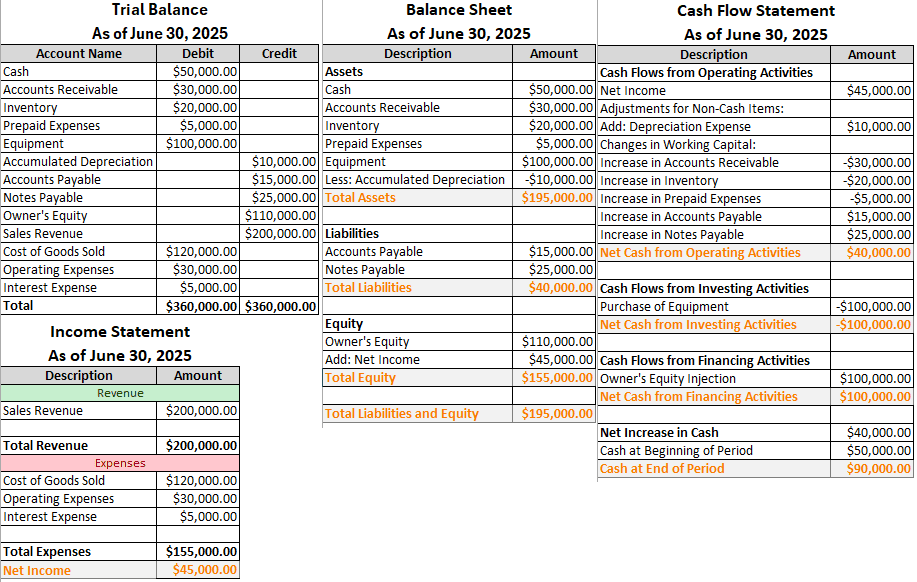
➤ Create three financial statements named Income Statement, Balance Sheet, and Cash Flow Statement.
➤ Add the revenues and subtract the expenses in the Income Statement.
➤ Balance the Assets with the Liabilities and Owner’s Equity in the Balance Sheet.
➤ Import data from the Trial Balance to the Cash Flow Statement to calculate the net increase in cash, and the financial statements will look like the following:
That must be confusing because there are actually a lot of things to be done in financial statements. To understand how to do this properly, you have to read the whole article. Therefore, open your dataset in Excel, and follow the instructions from this tutorial.
Preparing Financial Statements from Trial Balance
When talking about financial statements, it primarily refers to three sheets. Those are:
- Income Statement
- Balance Sheet
- Cash Flow Statement
This article assumes that you have a basic idea of how transactions work. There are lots of types of transactions that can happen in a company. It is not possible to include all of them in this article, so we chose the ones that are the most common for our trial balance. If you already know how to build the statements manually, it would be much easier for you to do it in excel.
Making the Income Statement
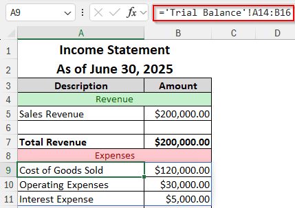
The income statement has essentially two parts: the revenues and the expenses. We will take the entries from the trial balance and prepare the sheet. Here is the format for the income statement:
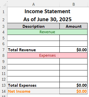
You might need to add more rows if you need, but for our dataset, these rows are enough. Here is how you insert entries:
Step 1: Calculate the Revenues
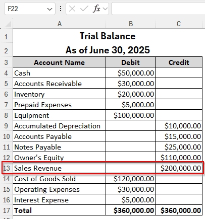
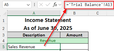
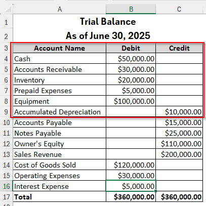
➤ First, we need to add the revenues. If we look at the Trial Balance, we have only one revenue in the C13 The name of the entry is Sales Revenue.
➤ In the A5 cell of our Income Statement, write this:
=’Trial Balance’!A13
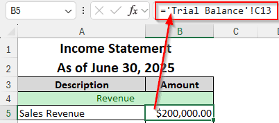
➤ In B5 cell, write this:
=’Trial Balance’!C13
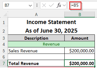
➤ In the B7 cell, we can just refer to the B5 cell, as there are no other entries for the revenue. Write the following formula to do that:
=B5
Step 2: Calculate the Expenses
➤ In the Trial Balance, there are three expenses, as shown in the picture below. We can refer to them in the income statement.
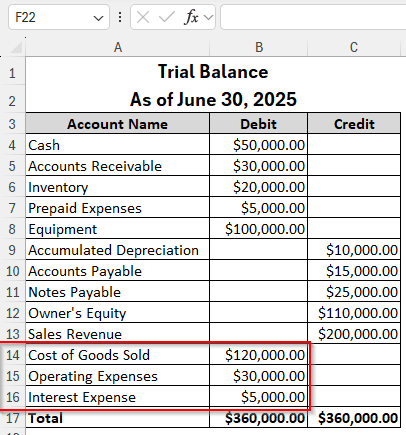
➤ Fortunately, these expenses are written one after another. Therefore, instead of referencing the cells one by one, we can spill the range in this table. Write this in the A9 cell of the Income Statement.
=’Trial Balance’!A14:B16
➤ For the Total Expenses, write this formula in the B13 cell to sum up:
=SUM(B9:B11)
Step 3: Calculate the Net Income
➤ Write this formula in the B14 cell for the net income calculation:
=B7-B13
Building the Balance Sheet
The balance sheet is used to prove the accounting equation A=L+O/E. From the equation, it is clear that there needs to be three sections in the balance sheet: the Assets, the Liabilities, and the Equity. We have built a spreadsheet for doing the calculation. Now let’s start inserting data:
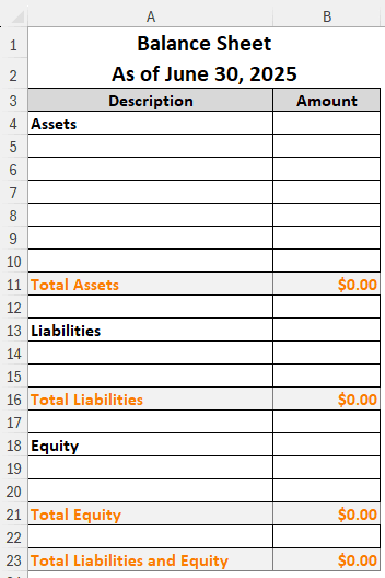
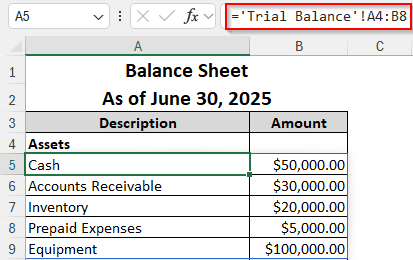
Step 1: Bring the Assets Over
➤ The marked section in the Trial Balance, minus the Accumulated Depreciation, will be added to the asset section.
➤ In the A5 cell of the Balance Sheet, write this formula:
=’Trial Balance’!A4:B8
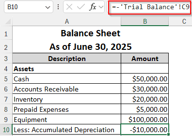
➤ The assets have been added. However, we need to subtract the Accumulated Depreciation. As it is being subtracted, we can write “Less: Accumulated Depreciation” for the description.
➤ To import the value from the Trial Balance, write this formula in the B10 cell:
=-‘Trial Balance’!C9
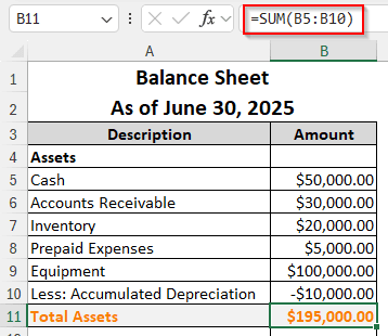
➤ Now, in order to calculate the total asset, use this formula in the B11 cell:
=SUM(B5:B10)
Step 2: Bring the Liabilities Over
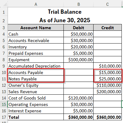
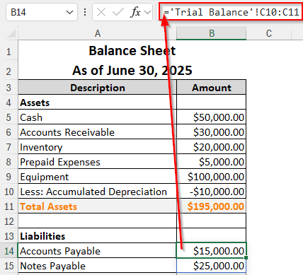
➤ For this case, as the liabilities are written in the credit section of the Trial Balance, they don’t match up with the column formatting of the Balance Sheet. Therefore, we have to import the descriptions and the amounts separately.
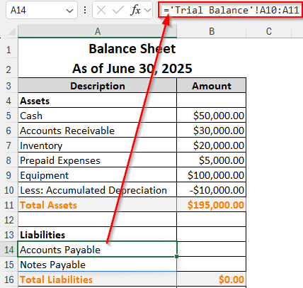
➤ To import the description, write this formula in the A14
=’Trial Balance’!A10:A11
➤ Now, to bring the values, write this formula in the B14 cell:
=’Trial Balance’!C10:C11
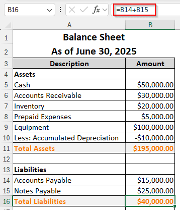
➤ Finally, add the values of the liabilities by writing this formula in the B16 cell:
=B14+B15
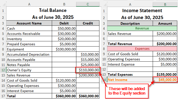
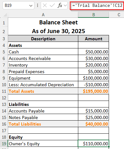
Step 3: Bring the Owner’s Equity
➤ There are essentially two things in the Equity The first one is from the Trial Balance, the current Owner’s Equity. The second one is from the Income statement, the Net Income.
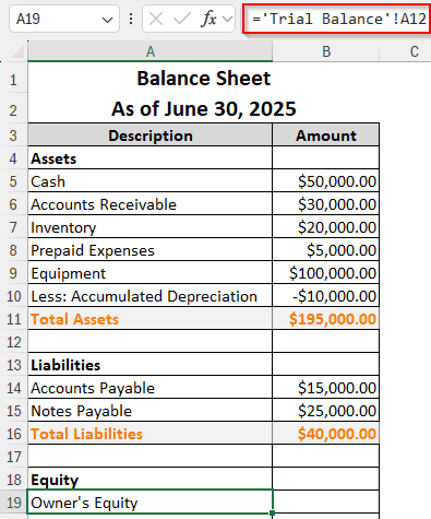
➤ First, we should bring from the Owner’s Equity. Write the following formula in A19 cell:
=’Trial Balance’!A12
➤ Write this formula in the B19 cell to import the amount:
=’Trial Balance’!C12
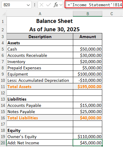
➤In the A20 cell, write “Add: Net Income”.
➤ In A21 cell, write this formula:
=’Income Statement’!B14
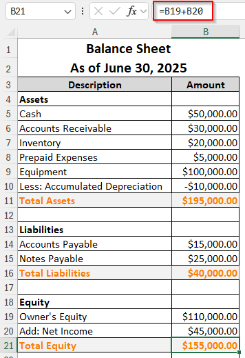
➤ Calculate the Total Equity using the following formula:
=B19+B20
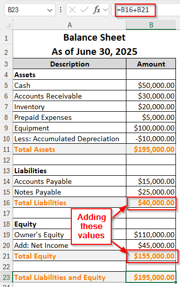
➤ Calculate the total liabilities and equity using the following formula in the B23 cell:
=B16+B21
Creating the Cash Flow Statement
This is the final financial statement that you would need to create. There will not be many shortcuts to import the values in this method; we mostly have to do it manually. Let’s see how to prepare the statement.
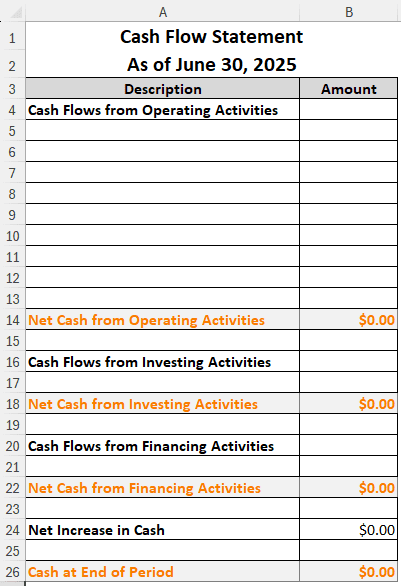
Step 1: Find the Cash Flow from Operating Activities
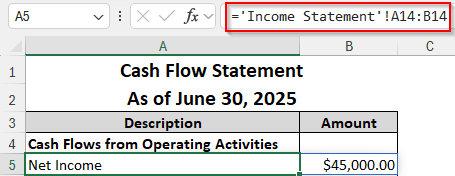
➤ Bring the Net Income from the Income statement by writing the following formula in the A5 cell:
=’Income Statement’!A14:B14
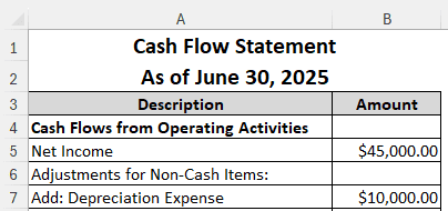
➤ Now, write “Adjustments for Non-Cash Items:” in A6 because we need to adjust the depreciation. The Accumulated Depreciation from the Trial Balance will be added by writing “Add: Depreciation Expense” in the A7 cell, and the value in B7.
➤ Then we add “Changes in Working Capital:” in the A8 The increases in the assets will be subtracted, and the increases in the payables will be added.
➤ Add the respective cells from the trial balance, and write Increase in in front of them.
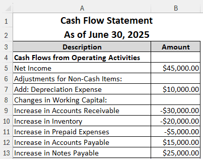
➤ Finally, calculate the net cash flow using this formula:
=SUM(B5:B13)
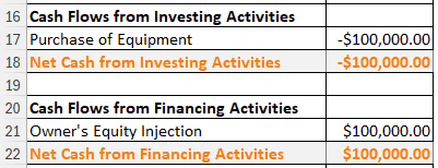
Step 2: Find the Cash Flow from Investing & Financing Activities
➤ Investment & Financing Activities both have one entry for them. We can write those entries and use the respective cell references.
➤ However, the investment needs to be subtracted, while the financing will be added.
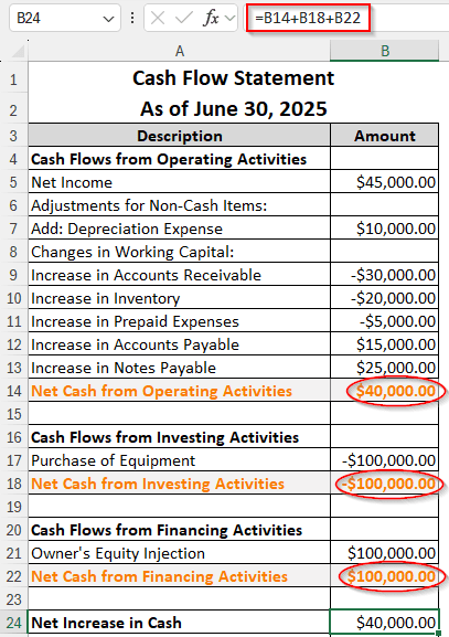
➤ To calculate the net increase in cash, use this formula:
=B14+B18+B22
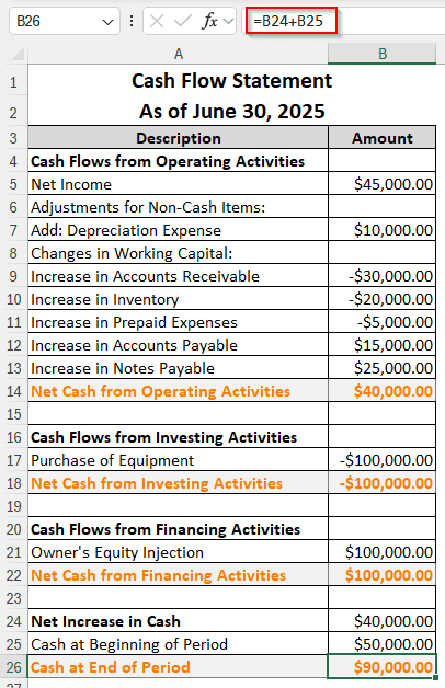
➤ In the row below, write the cash that was at the top of the Trial Balance. This is the Cash at Beginning of Period.
➤ Calculate the cash at the end of the period using this formula:
=B24+B25
Frequently Asked Questions
How to project financial statements in Excel?
Excel has built-in tools for forecasting data. Financial statements can be projected using the forecast sheet tool in Excel.
What is the formula for trial balance?
There is no formula for a trial balance, per se. However, the trial balance can be calculated by combining all the ledger entries into a single workbook and matching the debits and credits.
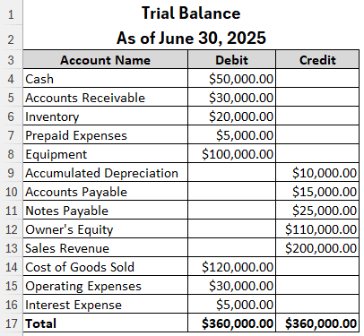
What does trial balance consist of?
The trial balance primarily consists of three columns. The first one is the name/description of the account, the second one is debit, and the third one is credit. According to the account type, the values are written in the debit or credit columns.
How to audit financial statements?
It is probably better to leave that to the auditor. However, the process usually involves gathering materials, analyzing data, verifying transactions, examining tax reports, and preparing the audit report.
Who prepares financial statements?
The directors of the company prepare financial statements or instruct the people under them to prepare the financial statements.
Wrapping Up
Preparing financial statements from the trial balance in Excel is not an easy job. We hope that we were able to make the task a bit easier for you. Should you have any questions, leave them in the comment section below. Download the workbook and you can use that as a template for your job.

