Pivot tables in Microsoft Excel allow easier calculation with formulas using calculated fields. After adding a calculated field, it might be required to edit it for corrections or other editorial purposes. In this article, we will learn how to edit a calculated field in a pivot table.
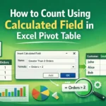
➤ Select any cell of the pivot table to enable the tabs related to the pivot table on the top bar.
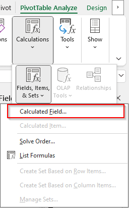
➤ Go to the PivotTable Analyze tab.
➤ Locate the Calculations group and open the dropdown menu of Fields, Items, & Sets. Select “Calculated Field” from there.
➤ You can edit the calculated fields by selecting one from the dropdown menu of the Name section and editing the Formula or the Name.
➤ Click Modify and OK to confirm the edit.
If that felt like a lot of steps, don’t worry, we will show the breakdown and explain each of the steps in this tutorial. Therefore, grab your spreadsheet and start following along to learn the method properly.
Steps to Edit Calculated Fields in Excel Pivot Table
For this tutorial, we have a dataset that has data about some salespeople. There are the names of the salespeople, their regions, the products they have sold, the number of units, and the revenues received.

In our pivot table, we want to calculate the price of each unit sold. As these salespeople are selling in different regions and to different buyers, the prices differ a lot. We will use a calculated field to do the job.
Step 1: Add a Calculated Field
Before editing the calculated field, we need to add one. Here is how we do that:
➤ First, we click any of the cells of the pivot table so that the PivotTable Analyze and Design tabs are enabled.
➤ Go to the PivotTable Analyze tab to find the Calculations group.
➤ From that group, open the Calculated Field button from the Fields, Items, & Sets option.
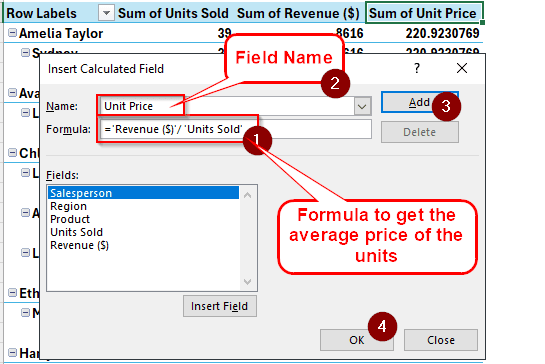
➤ A new window called “Insert Calculated Field” is opened. First, we change the We clear the edit box called Formula and write this formula there:
=’Revenue ($)’/ ‘Units Sold’
➤ Change the Name of the field to Unit Price.
➤ Press Add and OK to add the field.
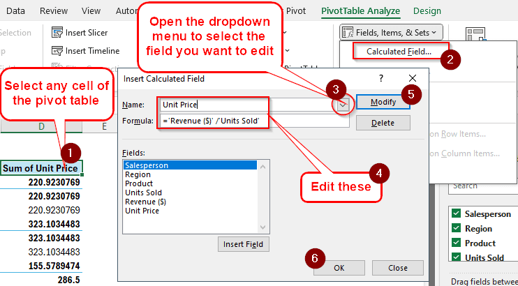
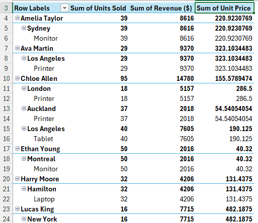
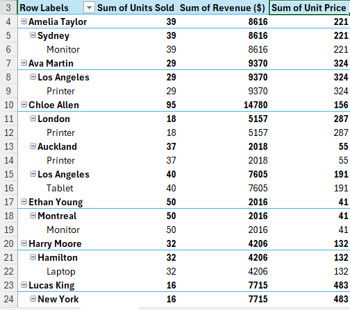
➤ The pivot table should look like this now:
Step 2: Edit the Calculated Field
In the previous step, we have created the calculated field we require. However, the unit prices are all fractions. We want the numbers to be integers. In order to do that, we need to edit the calculated field.
➤ Go to the Calculated Field section like we did in the previous step. In short, select a cell of the pivot table, go to the PivotTable Analyze tab, find Fields, Items, & Sets from the Calculations Click Calculated Field from the dropdown menu to open the window.
➤ Select the Unit Price by opening the dropdown menu of the edit box called Name.
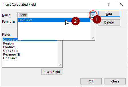
➤ Change the formula to the following:
= ROUNDUP( ‘Revenue ($)’/ ‘Units Sold’,0)
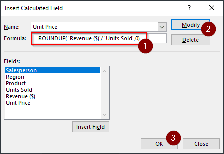
➤ Press Modify and OK.
➤ The calculated field has been modified. Now the pivot table will show the rounded-up unit prices.
Frequently Asked Questions
How do I edit fields in a PivotTable?
Select a cell of the pivot table to open the PivotTable Fields panel. To add a field, check the boxes of the field names. To remove those fields, just uncheck the boxes. To move the fields from Rows to Columns or vice versa, drag the fields using your mouse. It can be done for the Values area as well.
How to change calculated field name in PivotTable?
You can change the name in the sheet, and the pivot table will catch on. However, if you want to change it for real, you need to go to the Insert Calculated Field window and change the name. That will create a new calculated field. Delete the old field to make the new name stand out.
How do I update a field in a pivot table?
You can refresh the pivot table to update the field. You can go to the PivotTable Analyze tab and click Refresh from the Data group. Alternatively, you can press Alt+F5 or right-click on a cell and select Refresh.
What is the use of the calculated item in a pivot table?
Pivot tables generally provide some predefined calculations. However, that is often not enough for expert analysts. That is why Microsoft Excel has provided the calculated fields to do custom calculations in a pivot table.
How do I remove a formula from a PivotTable?
Click on the field from the Values section and select Remove Field. The calculation will be removed from the pivot table. However, if you want to remove a formula from the source table and then want it not to show up on the pivot table, just refresh the pivot table after altering the source table fields.
Wrapping Up
In this article, we have learned how to edit a calculated field in a pivot table. We hope that you have learned about calculated fields better from this tutorial. Download the practice sheet to try the method by yourself without touching any of your own spreadsheets. Leave a comment below with your feedback to let us know what you think.