Pivot tables allow you to format a table in various ways that regular tables cannot. Which is why, while pivot tables are mostly used for calculations, sometimes it might be required to display the actual values instead of calculations. In this article, we will learn how we can show actual value but not sum in pivot table.
➤ Make sure that the data in the pivot table is added to the data model.
➤ Right-click on the table from the PivotTable Fields section and add a measure.
➤ Name the measure and write this formula:
=CONCATENATEX(Table1, Table1[Month], “,”)
➤ Replace Table1 with the table name, Month with the field that you want to show the actual value of, and not the
➤ Organize the pivot table fields for your convenience.
Showing text in the pivot table values area is not a simple task by any means. Understanding the process from the key takeaways can indeed be difficult. Which is why we have broken the procedure into a lot of small steps so that you can understand the process properly. Therefore, keep reading the tutorial to understand the process better.
Showing Actual Value and Not Sum in Pivot Table
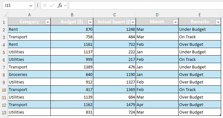
Here, we have the monthly budget information for four months. There are categories, budgets, the amount that was actually spent, the months, and remarks regarding the budget and the amount spent. What we want to do is show the categories as columns and the months as the values for the columns. Follow the steps below to accomplish the task.
Step 1: Create the Pivot Table
First of all, we need to create the pivot table you want to show the actual value without sums. Follow the procedure below to do so:
➤ Select the table, and go to the Insert tab.
➤ Click on PivotTable. While creating the new table, make sure to check the “Add this data to the Data Model” box.
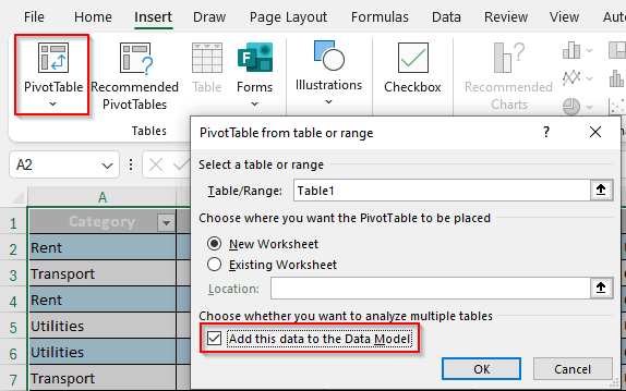
➤ Select all of the fields for the pivot table to show up

Step 2: Add a Measure
Now, we have to add our own measure so that Excel does not start counting the field that we want to show only the value of.
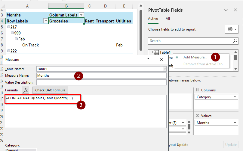
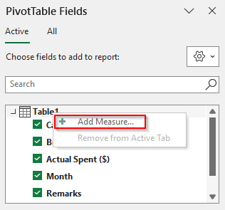
➤ From the PivotTable Fields section, right-click on the table and select Add Measure.
➤ Now, name the new measure. We are calling it Months as we want the month column to show up in value.
➤ Write this formula in the Formula section:
=CONCATENATEX(Table1,Table1[Month],”,”)
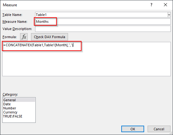
➤ Press OK to confirm.
Step 3: Organize the Pivot Table
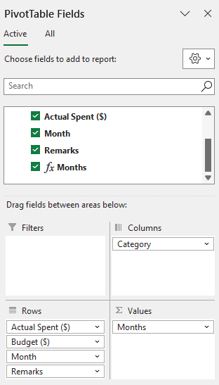
Now, we have added a field that Excel will refuse to sum up, and only show the values. We have to organize the pivot table now to make it look like the one we want. Follow the instructions below:
➤ Check the Months field if it isn’t checked yet.
➤ Move Category to the Columns area, as we want it to be our column.
➤ Move the Sum of Budget and the Sum of Actual Spent to rows. Those will now only show up as Budget and Actual Spent.
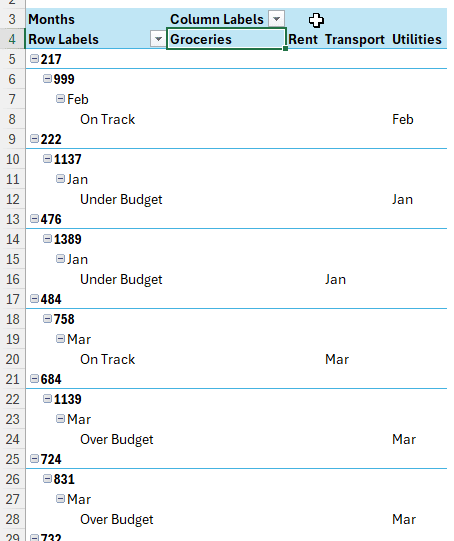
➤ In the end, the pivot table should look like the following:
Frequently Asked Questions
How to show actual values in pivot table instead of Sum?
It is not possible to show actual values instead of sums. However, you can show the counts, average, maximum/minimum values, multiplications, deviations/variances with/without the entire populations, etc.
How to get a pivot table to not Sum values?
Excel will automatically assign the fields in the Values area to sum. You can move these fields to other areas, like columns/rows/filters, to make them not sum up the values.
Why do pivots show count instead of the actual value?
Pivot tables are meant to do calculations. If you have columns that have numeric values, the table will show sums. If there are no numeric values, the value area will show counts instead.
How to change PivotTable values from sum to average?
Click on the Value Field Settings of the desired field from the Values section. From the “Summarize Values By“ tab, select Average and click OK. The value should now show average instead of sum.
How do I exclude values in a PivotTable?
You can remove the field from the Values area that you want to exclude to remove that from the pivot table. If you want to exclude individual values, uncheck the fields from the filters of each column in the table.
Wrapping Up
In this article, we have learned how to pivot table show actual value not sum in excel. We hope that you understand the process properly and will be able to create pivot tables without summations from now on. Leave a comment below if you face difficulties in any of the steps. Download the workbook and practice the procedure yourself to get good at it.