These days, pivot tables are often used in excel for data analysis. The process is not very straightforward, and people often struggle to create a proper pivot table with relationships and connections. In this article, we will learn how to create a pivot table from multiple tables in excel.
➤ Select each of the tables and press Ctrl+T to convert them into tables.
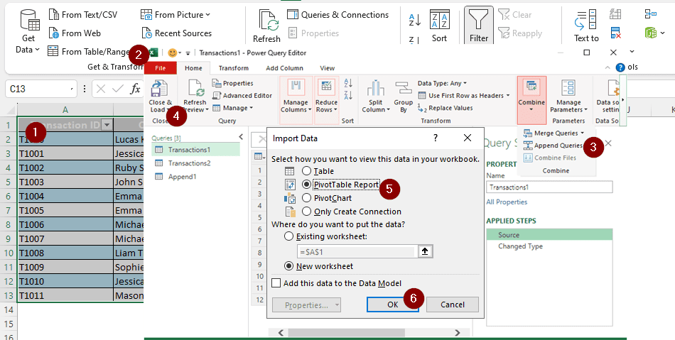
➤ Go to Data>Get & Transform Data>From Table/Range. Do the same for both tables.
➤ Combine the queries from Combine > Append Queries
➤ Click Close and Load To and select PivotTable Report
That might be confusing for a lot of people. Don’t worry, we have each step broken down along with images to help you make pivot tables for your dataset. Read till the end of the article, and if you have any questions, you can ask them in the comment section at the end of the tutorial.
Creating Pivot Table from Tables with Similar Columns
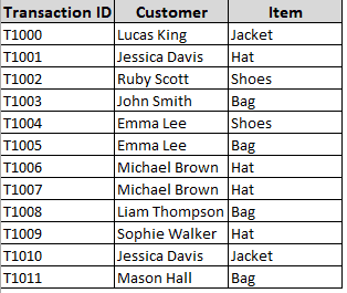
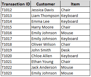
In this example, we have two tables with the same columns. There is some transaction data in those tables. Although the column headers are the same, the transactions aren’t. We have to combine these tables and create a new pivot table from them.
Step 1: Create Tables
We already have two tables here, but excel does not formally recognize them as tables. Those are just designed data points to excel. Here is how to do it:
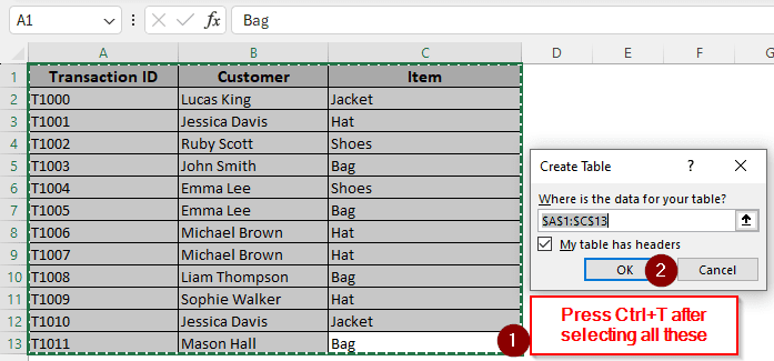
➤ Go to the first table, and select all the data.
➤ Then press Ctrl+T to create a table.
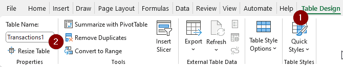
➤ From the “Table Design” tab, name the table something meaningful; it will help us later.
➤ Go to the second table and do the same.
Step 2: Add to Power Query
Now we need to load the tables into power query to create a connection and create a pivot table later.
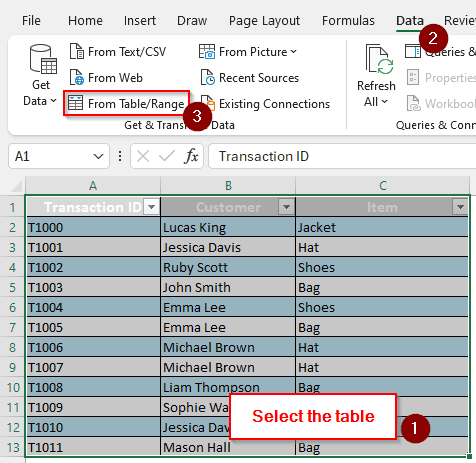
➤ Select all the data in a table, go to Data > From Table/Range
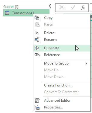
➤ From the “Power Query” window, duplicate the query.
Note:
We are duplicating this because it is easier, and we don’t have to go to the excel window again to import data. If you don’t want to do this, you can Get Data again for the other table.
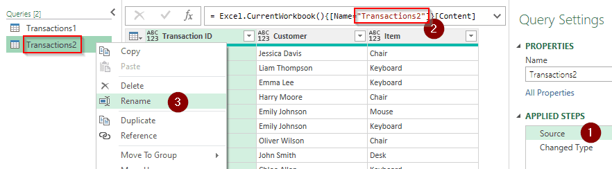
➤ In the new query, select Source from the right panel.
➤ In the formula bar, change the Name section to the name of the other table. This will make the query load data from that.
➤ From the left panel, rename the query according to the new table.
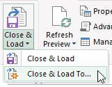
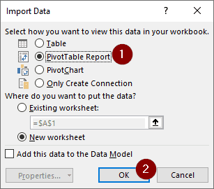
➤ Go to Close and Load > Close and Load To…
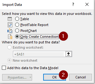
➤ From the “Import Data” dialog box, select “Only Create Connection” and press OK.
Step 3: Append Queries
Now, we have to merge the tables to create one pivot table from them.
➤ Double-click any of the tables from the Queries tab on the right to open the Power Query Editor

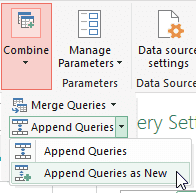
➤ Go to Combine > Append Queries > Append Queries as New
➤ Select both of the tables from the new dialog box and press OK.
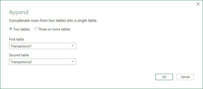
Note:
If you have more than two tables, you need to select “Three or more tables“ to select all the tables.
Step 4: Create a Pivot Table
Now it’s time for the final task. Follow the steps below:
➤ Click Close and Load > Close and Load To… This time, select PivotTable Report and press OK.
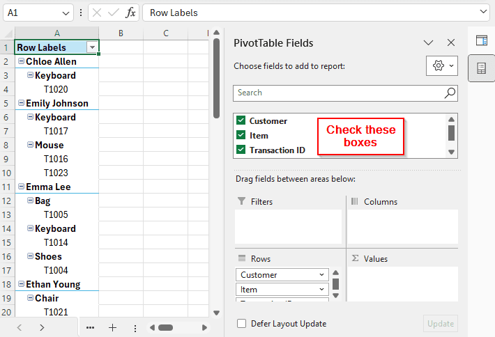
➤ From the new worksheet, go to the right panel, and select the column names you want to show up on your pivot table.
Pivot Table from Master Table and Transaction Table
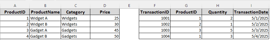
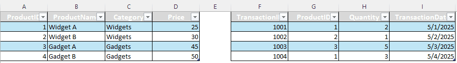
This time, we have two datasets with relations. The master table has some information about products, and the transaction table has some transaction data of those products. We are using a single sheet for both of those this time.
Step 1: Create Tables
You already know how to do this from method one, but here are the steps to refresh your memory:
➤ Select a table.
➤ Press Ctrl+T to create a table.
➤ Do this for the other table as well.
➤ Rename the tables from Table Design > Properties > Table Name
Step 2: Create a Relationship
The ProductID tabs match in both of the tables. We are going to create a relationship so that we can manage the data better in the pivot table.
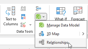
➤ Go to Data > Data Tools > Relationships
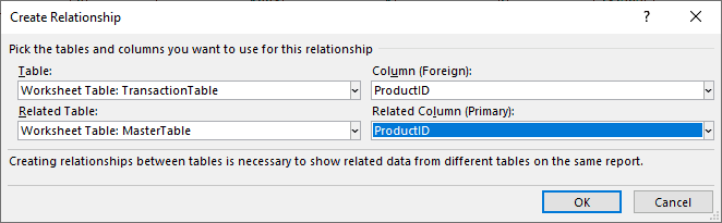
➤ From the “Manage Relationships” window, click New.
➤ The first table should be the table with the transactions and the related table should be the master table. Both of the columns are “ProductID” columns because they relate to each other.
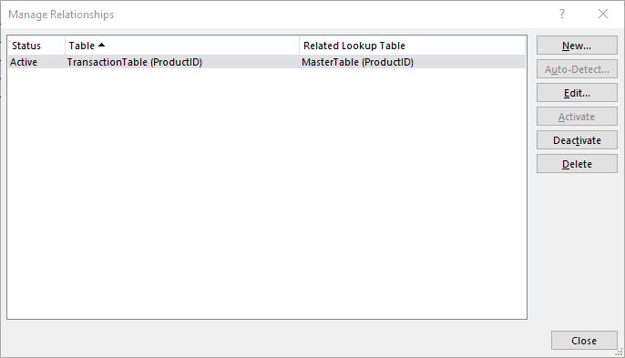
➤ Close the window
Step 3: Creating the Pivot Table
Now it is time to create the pivot table. Follow these steps sequentially:
➤ Go to the Insert tab, and select PivotTable>From Data Model
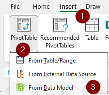
➤ Select New Worksheet and click OK

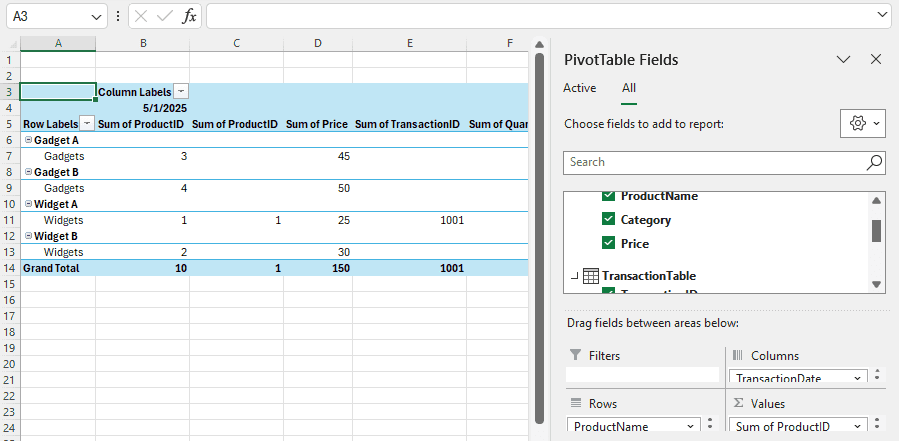
➤ Now you can select different fields from the pivot table you have created.
Frequently Asked Questions
How do I combine multiple tables into one table?
You can use regular copy and paste. Copy the table you want to merge using Ctrl+C and paste it next to the master table using Ctrl+V.
How to get data from a pivot table to another table?
From the Options menu, select Show Report Filter Pages. Then select the filter page you want to import, and press OK to get data from a pivot table to your worksheet.
How to automatically change data source in pivot table?
From the Analyze tab, select Change Data Source from the Data section. You can select the data source from there.
How to merge two data in Excel?
You can merge two cells in excel using the ampersand symbol (&). Write the formula like this: =A1 & B1. The output will merge both A1 and B1 cells.
How to sort a pivot table?
From the pivot table, click on the field where you want to sort the data. Then from the Data tab, click Sort, and select the options of sorting. Press OK to confirm.
Wrapping Up
In this article, we have learned two methods to create pivot table from multiple tables in excel. We hope that you have learned something from the tutorial and will be able to modify and use this for your own dataset. Leave a suggestion below, and we will see you next time in another tutorial.