Pivot tables are used for various kinds of data analysis. In a spreadsheet of student grades, a teacher might want to filter the top 10 students according to their numbers in a pivot table to decide the toppers in the class. In this article, we will learn how to show top 10 in pivot table in Excel.
➤ While in the compact layout (default view), go to the small arrow to the far right of Row Labels.
➤ Go to Value Filters > Top 10
➤ Customize the options if you need to, and Press OK
While that was easy, you might want to learn some advanced methods as well to become an expert at this. In this article, we will go in-depth to show you how to filter the top 10 with the help of a pivot table and VBA code. So, stick around to learn more and don’t forget to download the spreadsheet to follow along.
Showing Top 10 in Pivot Table
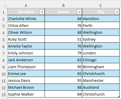
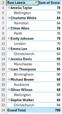
In this dataset, we have the scores of some students along with the cities they are from. We want to find the top 10 students among them based on their scores. Follow the procedure below to do so:
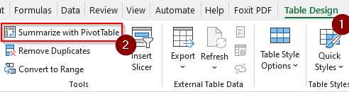
➤ First, convert the table to a pivot table by going to Table Design > Summarize with PivotTable.
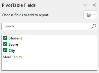
➤ After clicking OK, go to the pivot table in the new sheet and select all the fields from the PivotTable Fields section.
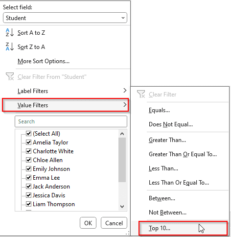
➤ From the pivot table, locate the small arrow to the right of the Row Labels. Usually, it is found in the A3 cell.
![]()
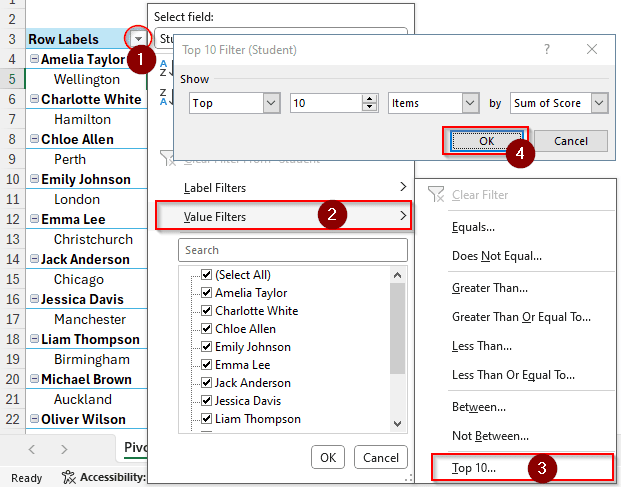
➤ Upon clicking on that, a submenu will open. From there, we go to Value Filters > Top 10…
➤ We keep the options as they are, as we want to show the top 10 by score.
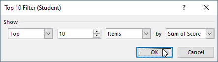
➤ Hit OK to show the result.
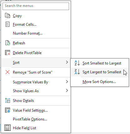
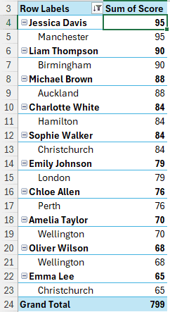
➤ Now, to show the top 10 in descending order, right-click on any number in the table.
➤ From the context menu, select Sort > Sort Largest to Smallest.
➤ The table should now be properly sorted, displaying the top 10 values of the pivot table.
Using VBA to Show Top 10 in Pivot Table
This time, we will take a different approach and separate the top 10 rows from the table before creating the pivot table. We will then create the pivot table from the new data range.
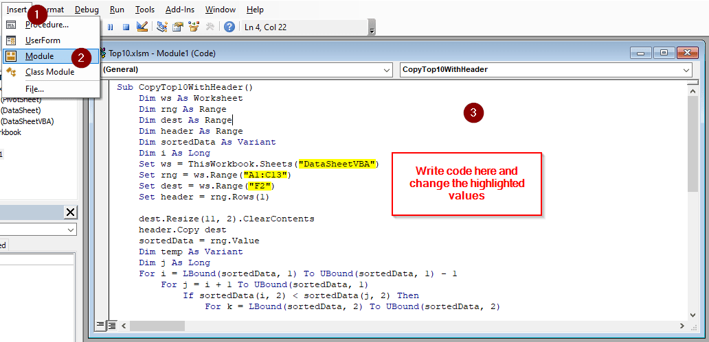
➤ Press Alt + F11 to open the Visual Basic window.
➤ Go to Insert > Module and write this code in the code window:
Sub CopyTop10WithHeader()
Dim ws As Worksheet
Dim rng As Range
Dim dest As Range
Dim header As Range
Dim sortedData As Variant
Dim i As Long
Set ws = ThisWorkbook.Sheets("DataSheetVBA")
Set rng = ws.Range("A1:C13")
Set dest = ws.Range("F2")
Set header = rng.Rows(1)
dest.Resize(11, 2).ClearContents
header.Copy dest
sortedData = rng.Value
Dim temp As Variant
Dim j As Long
For i = LBound(sortedData, 1) To UBound(sortedData, 1) - 1
For j = i + 1 To UBound(sortedData, 1)
If sortedData(i, 2) < sortedData(j, 2) Then
For k = LBound(sortedData, 2) To UBound(sortedData, 2)
temp = sortedData(i, k)
sortedData(i, k) = sortedData(j, k)
sortedData(j, k) = temp
Next k
End If
Next j
Next i
For i = 1 To Application.WorksheetFunction.Min(11, UBound(sortedData, 1))
For k = 1 To UBound(sortedData, 2)
dest.Offset(i - 1, k - 1).Value = sortedData(i, k)
Next k
Next i
header.Copy
dest.PasteSpecial Paste:=xlPasteFormats
Application.CutCopyMode = False
Dim sourceRange As Range
Set sourceRange = ws.Range(rng.Cells(2, 1), rng.Cells(Application.WorksheetFunction.Min(11, UBound(sortedData, 1) + 1), UBound(sortedData, 2)))
sourceRange.Copy
dest.Offset(1, 0).PasteSpecial Paste:=xlPasteFormats
Application.CutCopyMode = False
End Sub
➤ Replace DataSheetVBA with the name of your spreadsheet, A1:C13 with your range, and F2 with your new cell where you want to see the top 10 data.
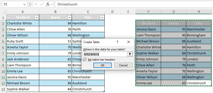
➤ Press F5 to run the code, then go back to your worksheet.
➤ Press Ctrl+T to turn the new dataset into a table.
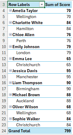
➤ Create a pivot table like we did in the previous method, and select all the fields as well.
➤ The final result will look like the one below; however, you can sort it in the pivot table using the right-click context menu, as we demonstrated earlier.
Frequently Asked Questions
How to show only top 10 in PivotTable in Google Sheets?
Open the pivot table editor and go to Filters. From there, click Add and choose the filter you will use to find the top 10 values. Then, select Filter by condition and choose Top 10.
How to get top 10 values in Excel?
Select the whole range of data from which you want to get the top 10 values. From the Data tab, select Filter. A filter option would be added to the columns. From the filter menu of the heading, go to Number Filters > Top 10.
How do I highlight top 10 values in Excel?
From the Style group of the Home tab, open the dropdown menu of Conditional Formatting. From there, go to Top/Bottom Rules > Top 10 Items. Select the formatting of the highlight and hit OK.
How to get top 5 in pivot table?
From the first method in this article, follow the technique until you click on Top 10. From the Top 10 Filter window, write 5 in the second edit box, and click OK to get the top 5 in the pivot table.
How to rank in Excel?
The rank function ranks a value from a list of values, which is helpful for finding the top 10 or other rankings within a list. The function takes 3 parameters. The first parameter is the input cell that you want to rank. The second parameter is the series of values from which it will rank. The third one is a boolean value, where 0 represents descending and 1 represents ascending. The function is written like this:
=RANK(A1, A:A, 0)
This formula finds the rank of the A1 cell in column A in descending order.
Wrapping Up
From this article, we have learned how to show top 10 in pivot table manually and with VBA coding. Hope you were able to gain some knowledge from the tutorial. If you like the tutorial, consider bookmarking the site and leaving some suggestions for us below.