Adding a sorted drop-down on the column heading makes repetitive entries faster and reduces human errors. To sort a drop-down in Excel, you can use the Data Validation tool.
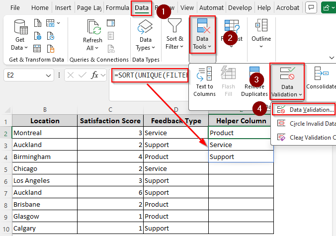
➤ Create a helper column and select a cell where you want to put the list for the drop-down. We’re selecting cell E2. Enter the following formula:
=SORT(UNIQUE(FILTER(D2:D10)))
➤ Instead of D2:D10 put your original data range based on which you’re creating the sorted drop-down.
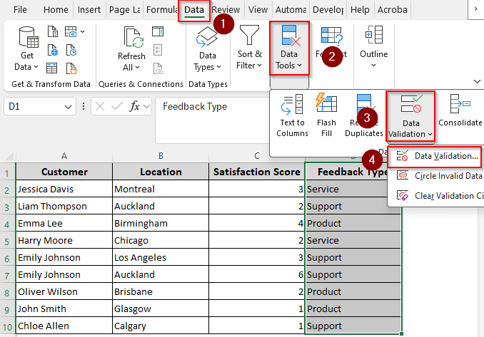
➤ Select the cell to enter a drop-down and go to the Data tab >> Data Validation >> Data Validation.
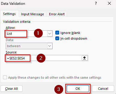
➤ In the Data Validation dialog box, choose List from the Allow box. In the Source box, enter the reference to the cell where your SORT formula starts, followed by a hash (#). We entered =$E$2# for our dataset. Click Ok.
While this is the easiest way to sort a drop-down alphabetically or numerically, it’s only available for the newer version of Excel. In this article, we’ll cover more methods such as using the Define Name feature, the Power Query tool, and VBA coding suitable for old and new Excel versions.
Manually Sort Source Data and Add a Drop-Down
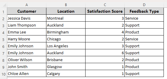
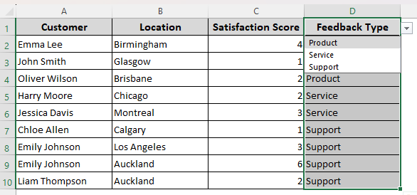
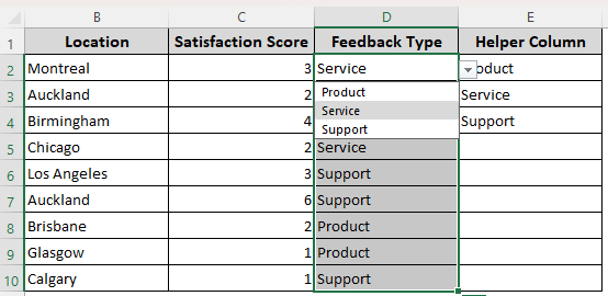
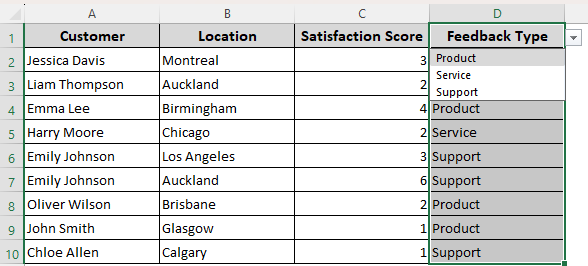
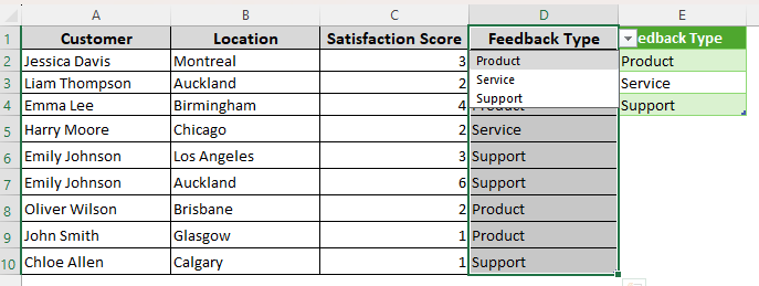
To demonstrate the methods, we’ll use the following dataset with columns for customer name,location, and other info. In column D, we have some repetitive values. Based on the data in column D, we’ll add a drop-down list on the column heading.
If you don’t mind sorting your original data source in alphabetical or numerical order, you can use this manual sorting method. The main drawback of this method is that the changes are static, so the new entries aren’t sorted automatically.
Avoid this if you want to protect the original order of your dataset and want dynamic changes. Here’s the process:
➤ Select your full data range, go to the Data tab, and click Sort from the Sort & Filter group.
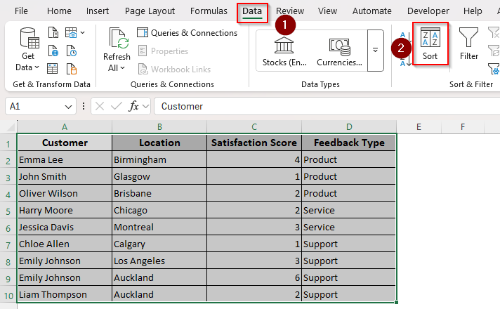
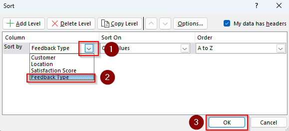
➤ From the Sort dialog box, click on the Sort By drop-down and select the column where you’re adding the drop-down. Press Ok.
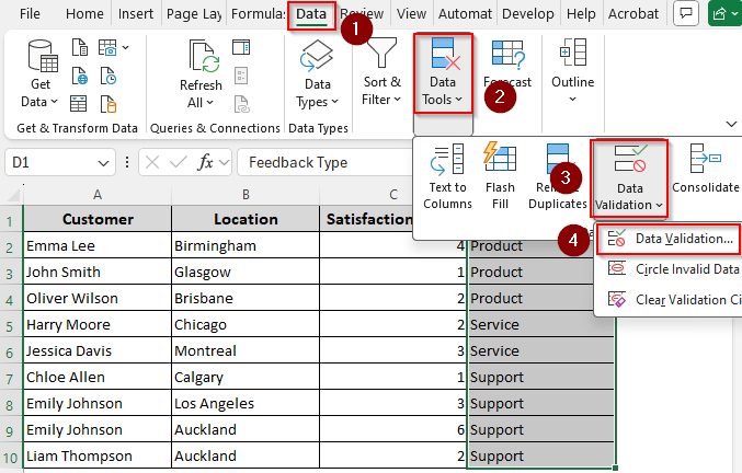
➤ Now, highlight the range where you want to add the drop-down list (including the header). Go to the Data Tools group and click the Data Validation option. Select Data Validation from the drop-down menu.
➤ As the Data Validation dialog box appears, click on the drop-down arrow on the Allow field and choose List.
➤ In the Source box, click on the upward arrow sign and select the cells with the source data for the drop-down list (without the header).
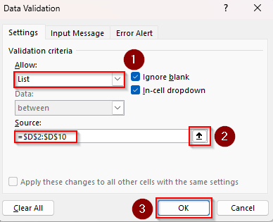
➤ Finally, press Ok and Excel will add a drop-down on the header cell with alphabetically sorted data.
Using the SORT Function and Data Validation
In Excel 365/2021, the SORT function returns a sorted version of a range or array. It automatically fills multiple cells with results which is also known as Spill Range. If you want to remove duplicates and blank cells, you can combine it with the UNIQUE and FILTER functions.
We’ll use all three functions to sort data in a helper column and use it as our reference for the drop-down. Here are the steps:
➤ Create helper columns to input the sorted data for a drop-down list. As we’re only working with column D, we created only one helper column (column E).
➤ In the first cell of the helper column, enter the following formula:
=SORT(UNIQUE(FILTER(D2:D10, D2:D10<>””)))
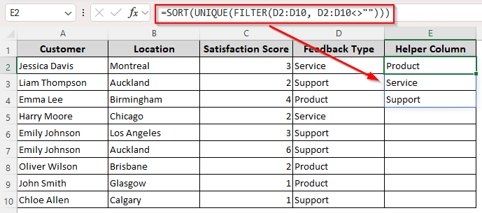
➤ Replace D2:D10 with your original source data range. Excel will return a spill range with sorted data and exclude the duplicates and blank cells. You can use the SORT() function only if your data doesn’t have duplicates or blank cells.
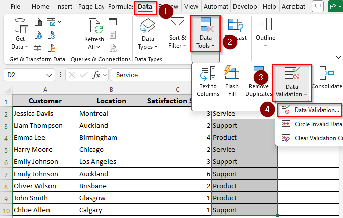
➤ Now, select your original data range including the heading where you want to add the drop-down list and go to the Data tab >> Data Validation >> Data Validation.
➤ From the Data Validation dialog box, click on the Allow drop-down and select List.
➤ In the Source box, enter the reference of the helper column cell where you entered the sorted data followed by a hash(#) symbol.
➤ For example, we entered =$E$2# in the Source box.
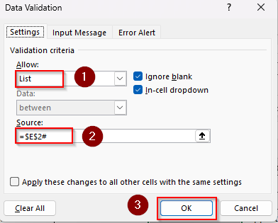
➤ Click Ok and Excel will now add a sorted drop-down list on the heading cell of your original data range.
Applying the COUNTA and OFFSET Functions with a Defined Name
In older versions of Excel (before 2021), the SORT function isn’t available. So, we need to follow a roundabout way using the OFFSET and COUNTA. The functions create a dynamic range of your selected data excluding the empty cells.
In this case, we’ll sort and enter our reference data in a different sheet. Below are the steps:
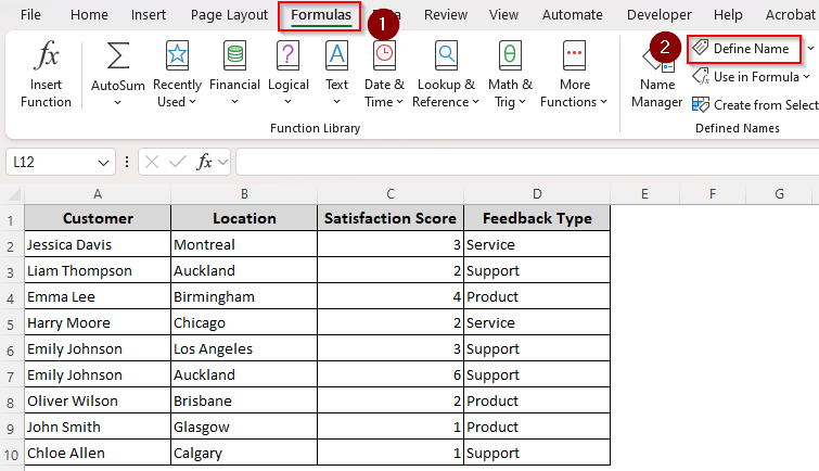
➤ Start by highlighting your data range. From the main ribbon, open the Formulas tab and select the Define Name option from the Defined Names group.
➤ As the New Name dialog box opens, enter your preferred name for your data range in the Name field. We entered MyRange for our dataset.
➤ Enter the following formula in the Refers To box:
=OFFSET(Sheet3!$D$2, 0, 0, COUNTA(Sheet3!$D$2:$D$10))
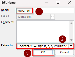
➤ Here, Sheet3!$D$2 is the reference (starting point) of your list. We start at D2 as D1 is a header which is not part of the actual list items. Replace the values based on your original dataset.
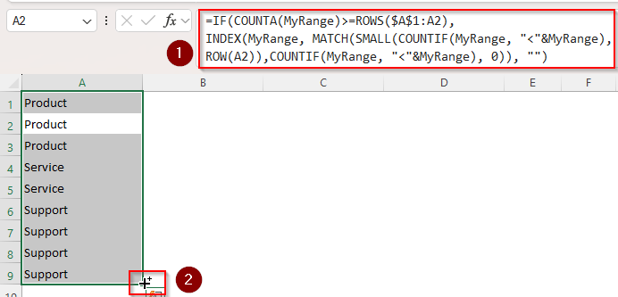
➤ To create your reference range, open a new sheet (Sheet4), and enter the following formula in its first cell (A1):
=IF(COUNTA(MyRange)>=ROWS($A$1:A1), INDEX(MyRange, MATCH(SMALL(COUNTIF(MyRange, “<“&MyRange), ROW(A1)),COUNTIF(MyRange, “<“&MyRange), 0)), “”)
➤ Replace MyRange with the defined name you used in the previous steps. This formula returns the values in MyRange sorted in ascending order.
➤ Use the fill handle (+ sign) in cell A1 to extend the full list.
➤ Go back to Sheet3 and select your original data range with the heading. Open the Data tab >> Data Validation >> Data Validation.
➤ From the Allow field, choose List. In the Source field, enter the reference data range from the second sheet.
➤ For example, we entered =Sheet4!$A$1:$A$9 for our dataset.
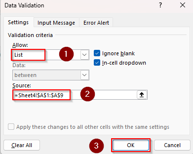
➤ Finally, press Ok. Here’s the result:
Sorting Reference Data with Power Query
You can use Power Query to sort your reference data and put it in a different location on the same sheet or a different sheet. Later on, use the Data Validation feature to create the drop-down list based on this data. Here are the details:
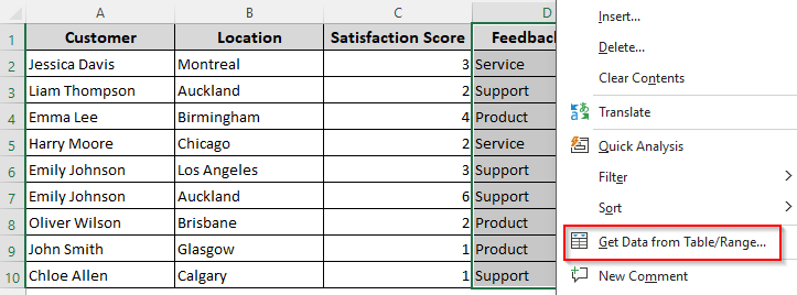
➤ Select your data range for the drop-down and right-click on your mouse. Select Get Data From Table or Range from the menu.
➤ When Excel prompts to create a table, press Ok.
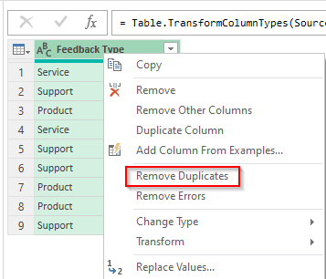
➤ In the Power Query Editor, right-click on the table and select Remove Duplicates.
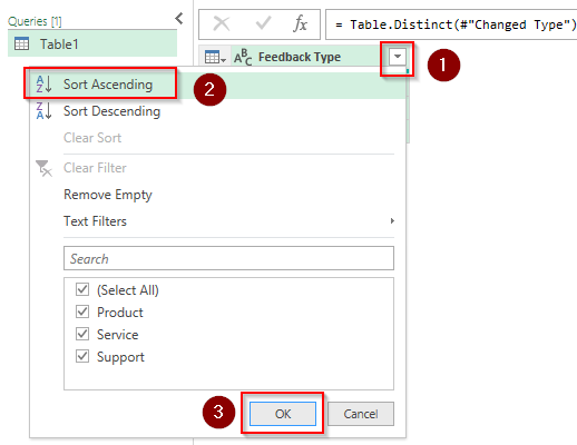
➤ After that, click on the downward arrow on the column heading, choose Sort Ascending from the menu, and press Ok. Your reference data for the drop-down list is now ready.
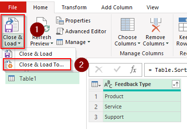
➤ Click on the downward arrow on the Close & Load To option from the top ribbon.
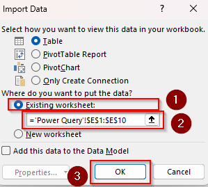
➤ Select the Existing Worksheet option from the list and choose a location to input the sorted data. Press Ok.
➤ Now, select your original data range to add the drop-down list. Go to the Data tab >> Data Validation >> Data Validation.
➤ In the Allow box, select List. As for the Source box, enter the reference data range extracted from Power Query.
➤ Click Ok and the final result should look like this:
Sort Drop Down with Custom VBA Macro
With a VBA macro, we can easily add a drop-down list with our selected sorted data. Follow the steps given below:
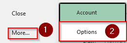
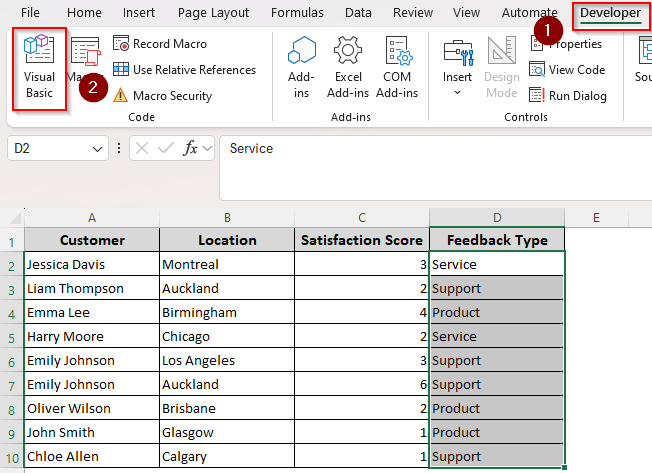
➤ First, check if you can find the Developer tab on the main ribbon. If not, go to the File tab >> More >> Options.
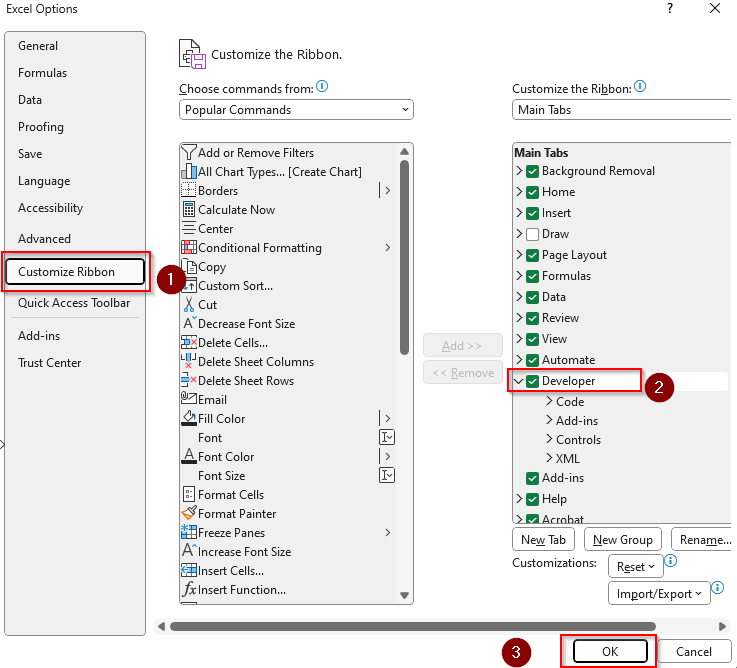
➤ From the side column, choose Customize Ribbon and select the Developer option from the last column. Click Ok.
➤ Now, select your data range and go to the Developer tab. Click on Visual Basic to open the VBA Editor.
➤ Click on Insert and select Module from the menu to create a new module.
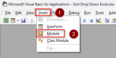
➤ In the blank field, paste the following code:
Sub AddSortedDropdownToSelectedRange()
Dim dropDownRange As Range
Dim sourceRange As Range
Dim cell As Range
Dim dict As Object
Dim val As Variant
Dim sortedList As Variant
Dim dropDownString As String
Dim i As Long
' Get the pre-selected range (where drop-downs will be applied)
Set dropDownRange = Selection
If dropDownRange Is Nothing Then
MsgBox "Please select the range where drop-downs should be added before running the macro.", vbExclamation
Exit Sub
End If
' Prompt user to select the range from which to build the drop-down values
On Error Resume Next
Set sourceRange = Application.InputBox("Select the data range to generate the drop-down list from (excluding headers):", Type:=8)
On Error GoTo 0
If sourceRange Is Nothing Then
MsgBox "No source range selected. Exiting."
Exit Sub
End If
' Create dictionary to collect unique values
Set dict = CreateObject("Scripting.Dictionary")
For Each cell In sourceRange
val = Trim(cell.value)
If Len(val) > 0 Then
If Not dict.exists(val) Then
dict.Add val, 1
End If
End If
Next cell
If dict.Count = 0 Then
MsgBox "No unique values found in the source range.", vbExclamation
Exit Sub
End If
' Sort the dictionary keys
sortedList = dict.keys
Call QuickSort(sortedList, LBound(sortedList), UBound(sortedList))
' Create comma-separated drop-down string
For i = LBound(sortedList) To UBound(sortedList)
dropDownString = dropDownString & sortedList(i) & ","
Next i
dropDownString = Left(dropDownString, Len(dropDownString) - 1)
' Apply drop-downs to each cell in the selected (header) range
For Each cell In dropDownRange
With cell.Validation
.Delete
.Add Type:=xlValidateList, AlertStyle:=xlValidAlertStop, _
Operator:=xlBetween, Formula1:=dropDownString
.IgnoreBlank = True
.InCellDropdown = True
.ShowInput = True
.ShowError = True
End With
Next cell
MsgBox "Sorted drop-downs added to the selected range!", vbInformation
End Sub
' Helper: QuickSort implementation for sorting arrays
Sub QuickSort(arr As Variant, first As Long, last As Long)
Dim low As Long, high As Long
Dim mid As Variant, temp As Variant
low = first
high = last
mid = arr((first + last) \ 2)
Do While low <= high
Do While arr(low) < mid
low = low + 1
Loop
Do While arr(high) > mid
high = high - 1
Loop
If low <= high Then
temp = arr(low)
arr(low) = arr(high)
arr(high) = temp
low = low + 1
high = high - 1
End If
Loop
If first < high Then QuickSort arr, first, high
If low < last Then QuickSort arr, low, last
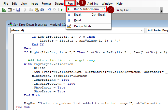
End Sub➤ Press F5 or click on Run and choose Run Sub/UserForm from the drop-down menu. If Excel prompts to add a macro name, press Ok.
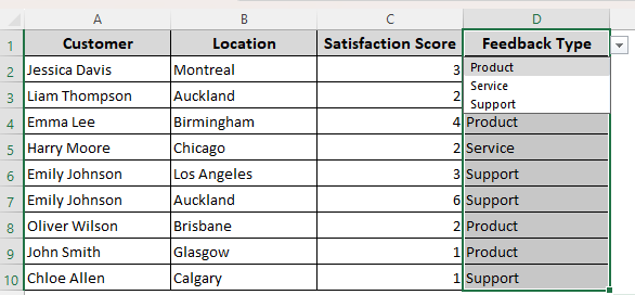
➤ Now, go back to the Excel tab and select the data range to sort and create a drop-down list based on it. Once done, the list should look like this:
➤ Before closing the file,when Excel prompts to save the changes, make sure to press Save.
Frequently Asked Questions
How do you sort based on a custom list in Excel?
Go to the File tab >> More >> Options >> Advanced >> General >> Edit Custom Lists.
When the Custom Lists box arrives, click on New List. In the List Entries field, enter the items you want to add in your custom list. After entering each item, press Enter on your keyboard. Click Add. When sorting your data, click on the Order drop-down, select Custom List, and choose the list you created.
How do I manually create a drop-down list in Excel?
Select the cell(s) where you want the drop-down. Go to the Data tab >> Data Validation >> Data Validation. In the Data Validation dialog box, select List from the Allow drop-down. Go to the Source box, type your items, separated by commas without any spaces. For example, type Yes,No,Later. Press Ok.
How do I move a drop-down list in Excel?
Right-click on the cell with your drop-down and choose Copy. Or, simply press CTRL + C . Right-click on a new cell where you want to move the drop-down list. Choose Paste Special, click on the Validation option, and press Ok.
How to delete a drop-down list?
Select the cell that has the drop-down list. Go to the Data tab >> Data Validation >> Data Validation. In the dialog box, click Clear All. Finally, click OK.
Concluding Words
Sorting a drop-down list in Excel can be a little complex no matter which method you choose. Usually, you need to put the sorted data in a different location (preferably a different sheet) and use it as a reference for the drop-down list.
For the sorting, it’s best to use the SORT() function or the Power Query tool. Later, use Data Validation to add a drop-down list based on the reference data you select.