Pivot tables are a powerful tool that helps you summarize, analyze, and explore data interactively. In Google Sheets, you can use pivot tables to extract insights from large datasets without writing complex formulas, making them ideal for reporting, trend analysis, and data exploration.
This article outlines the most effective methods for creating and using pivot tables in Google Sheets, including how to analyze large datasets and how to build pivot tables from multiple sheets.
Steps to build a Pivot Table in Google Sheets for summarizing sales data by product:
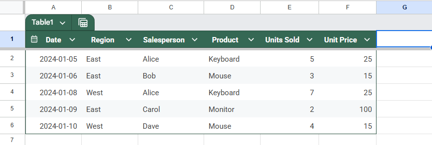
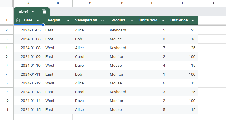
➤ Select the range A1:F6, which includes columns like Date, Region, Salesperson, Product, Units Sold, and Unit Price.
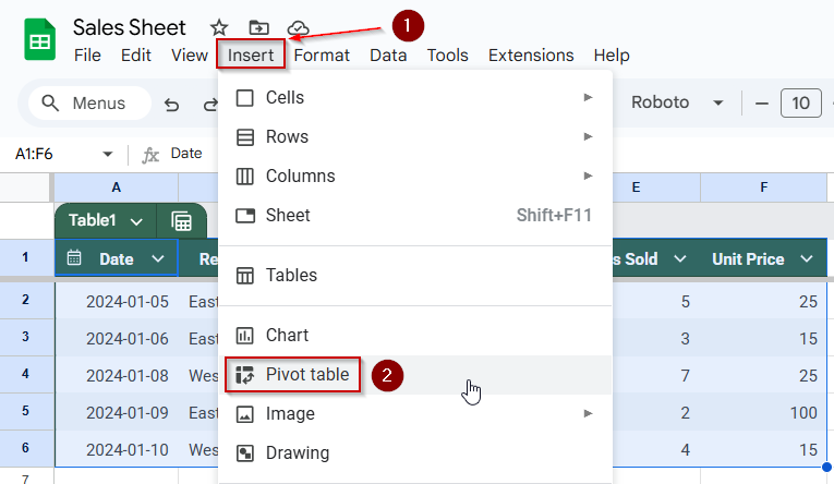
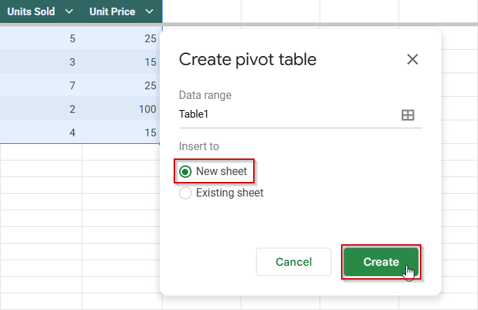
➤ Go to Insert >> Pivot table and choose “New sheet” as the location.
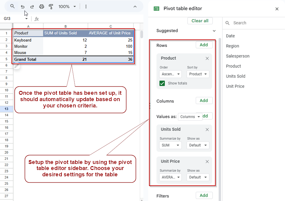
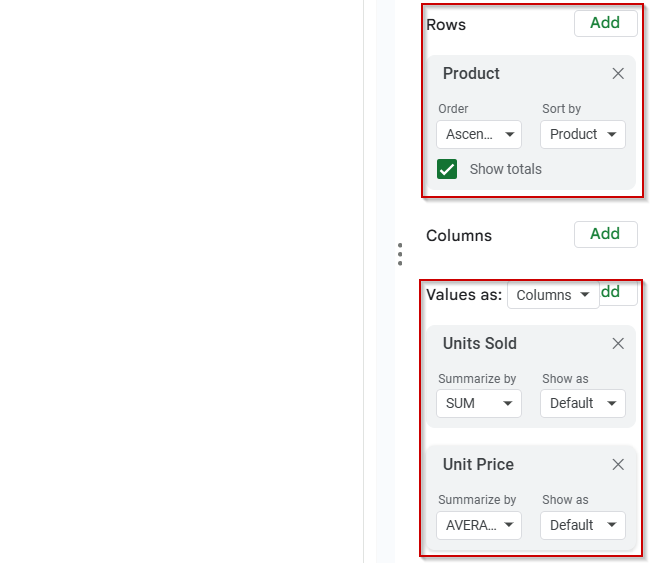
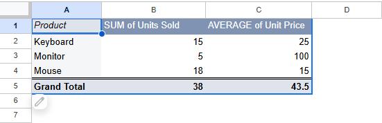
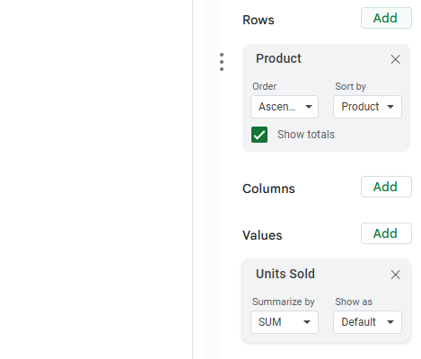
➤ In the Pivot Table Editor, under Rows, add Product to group data by item.
➤ Under Values, add Units Sold, summarized by SUM to calculate total sales volume.
➤ Optionally, add Unit Price to Values, summarized by AVERAGE for pricing insights.
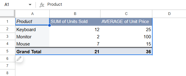
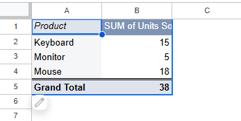
➤ Review the pivot table to instantly see which products sold the most and analyze performance efficiently.
What is a Pivot Table in Google Sheets?
A pivot table in Google Sheets is a dynamic summary tool that allows you to group, filter, and calculate data from a larger dataset. It helps you analyze patterns and trends by rearranging data interactively, hence the term “pivot.”
For example, instead of manually scanning through hundreds of sales records, you can use a pivot table to calculate total sales by month instantly, average order value by region, or the number of orders per salesperson. It’s especially useful for summarizing large datasets without writing any formulas. Let’s walk through how to create a basic pivot table in Google Sheets.
Build a Basic Pivot Table to Summarize Sales Data
Pivot tables are ideal for summarizing large datasets into meaningful insights without writing formulas. In this method, you’ll learn how to use Google Sheets’ built-in Pivot Table tool to calculate total units sold per product. This is especially useful for sales analysis, allowing you to identify top-performing products with just a few clicks.
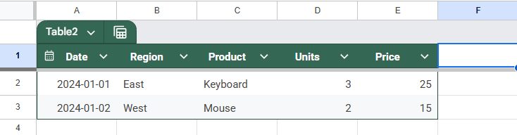
This is the dataset we will be using to demonstrate the methods.
Steps:
➤ Select the range A1:F6
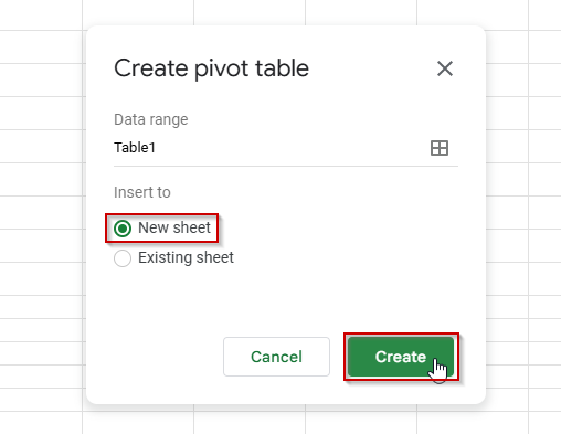
➤ Go to Insert >> Pivot table
➤ Choose “New sheet” as the location and click Create
➤ In the Pivot Table Editor:
- Rows: Add Product
- Values: Add Units Sold (summarized by SUM)
- Values: Optionally add Unit Price (summarized by AVERAGE)
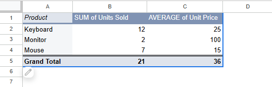
➤ Your pivot table will now display total units sold per product, allowing for a quick and clean analysis of product performance.
Combine and Analyze Data from Multiple Sheets Using a Pivot Table
When your data is split across multiple sheets, such as monthly sales reports, you can still create a single pivot table to analyze it all together. Although Google Sheets doesn’t allow direct multi-sheet pivot tables, you can work around this by first consolidating the data using formulas like QUERY. Once your data is merged into one table, you can use a pivot table to summarize and compare performance across different periods or categories. This method is useful for multi-month, multi-department, or multi-source reporting.
Create Two Source Sheets
Let’s say we create a sales sheet for January and another for February.
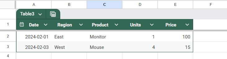
First sheet: Sales_Jan
Second sheet: Sales_Feb
Combine Data in a New Sheet
In a third sheet called Combined_Data, enter the following formula in cell A1:
={“Date”,”Region”,”Product”,”Units”,”Price”; QUERY({Sales_Jan!A2:E; Sales_Feb!A2:E}, “SELECT * WHERE Col1 IS NOT NULL”, 0)}
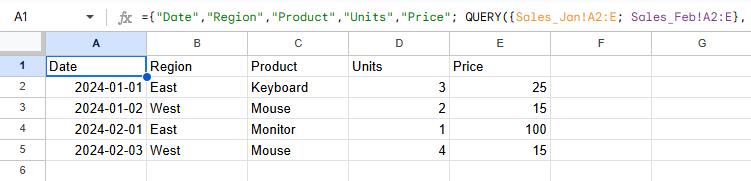
The QUERY function combines data from two sheets, Sales_Jan and Sales_Feb, and filters out empty rows to prepare a clean dataset for analysis (like a pivot table).
This merges two data ranges vertically (stacking one below the other). It pulls all columns A to E from both sheets, starting from row 2 (to skip headers).
➧ SELECT * WHERE Col1 IS NOT NULL:
This is a SQL-style query that means:
SELECT *: Return all columns
WHERE Col1 IS NOT NULL: Only include rows where the first column (Date) is not blank (removes any extra empty rows)
➧ 0
This tells Google Sheets that the data does not have a header row inside the query range. It treats all rows equally, so headers must exist outside the formula (i.e., manually added).
Create Pivot Table from Combined Sheet
➤ Select the range starting from A1 in the Combined_Data sheet
➤ Go to Insert >> Pivot table
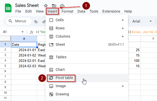
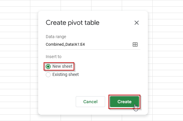
➤ Choose New sheet and click Create
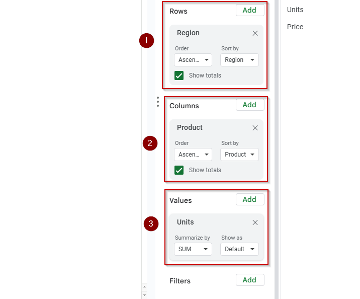
➤ In the Pivot Table Editor:
- Rows: Add Region
- Columns: Add Product
- Values: Add Units (summarize by SUM)
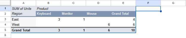
Now you have a pivot table that compares total units sold by region and product across both January and February.
Refresh a Pivot Table After Updating Source Data
When you edit or expand your original dataset, your pivot table in Google Sheets may not reflect those changes immediately. This method shows how to refresh the pivot table or update its data range if you’ve added new rows or columns.
Steps:
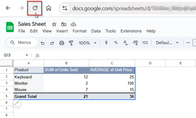
➤ If you’ve only edited existing values in your dataset, click the Refresh icon in your browser. Google Sheets will automatically update the pivot table with the new values.
➤ If you’ve added new rows or columns to the source data, you must manually update the pivot table range.
➤ Hover over the pivot table and click Edit to open the Pivot Table Editor on the right.
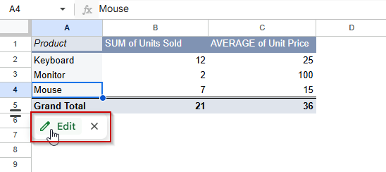
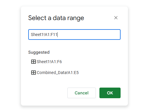
➤ Under Data range, adjust the range to include the new rows or columns. For example, update A1:F6 to A1:F11.
➤ The pivot table will now reflect the expanded dataset, including any new entries.
This ensures your pivot analysis remains accurate even as your source data grows or changes.
Add Filters and Slicers to a Pivot Table for Interactive Analysis
Filters and slicers allow you to dynamically explore and narrow down your pivot table results. While filters are set inside the Pivot Table Editor, slicers provide a clickable tool right on your sheet. This method helps you drill into data by fields like region or salesperson, making your analysis more interactive and presentation-ready.
We will use this dataset for this method.
Steps:
➤ Select the range A1:F11 (including headers and all 10 rows of data)
➤ Go to Insert >> Pivot Table, choose “New sheet”, and click Create
Set Up Your Pivot Table:
➤ In the Pivot Table Editor:
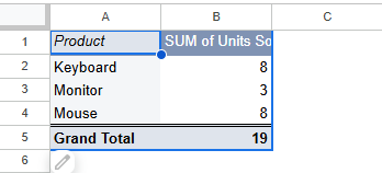
- Rows: Add Product
- Values: Add Units Sold (Summarize by SUM)
You’ll now see a table summarizing the number of units sold per product.
Adding a Filter
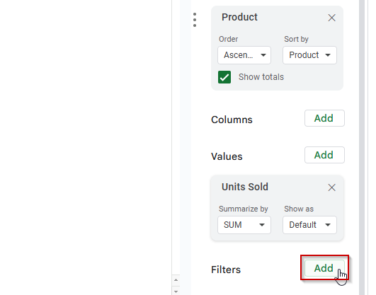
➤ In the Pivot Table Editor, scroll to Filters >> Add
➤ Choose Region
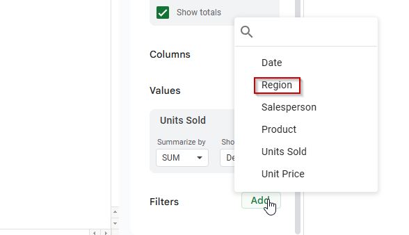
➤ Use the checkboxes to show only East, West, or both regions.
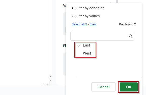
The pivot table will update accordingly.
Adding a Slicer
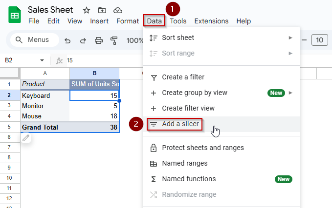
➤ Click anywhere inside the pivot table
➤ Go to Data >> Add a slicer
➤ In the Slicer panel on the right, set the slicer to column Salesperson
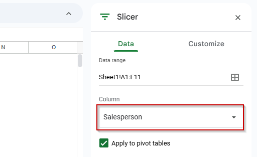
➤ Drag the slicer box wherever you want on your sheet
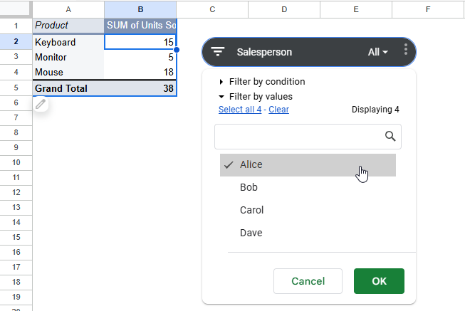
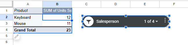
Now, you (or stakeholders) can click to filter by salesperson in real-time, without needing to reopen the Pivot Table Editor.
Frequently Asked Questions
What is a pivot table in Google Sheets used for?
A pivot table summarizes large data sets, allowing you to group, count, and analyze information quickly, such as totals by category, date, region, or other dimensions.
Can you create a pivot table from multiple sheets in Google Sheets?
Yes, but you must first combine the data using QUERY, ARRAYFORMULA, or curly brackets {} into one sheet before building the pivot table.
How do I refresh a pivot table in Google Sheets?
Pivot tables in Google Sheets update automatically when source data changes. Just reopen the file or click into the pivot to force a refresh if needed.
How do I remove grand totals from a pivot table?
Open the Pivot Table Editor, go to the Values section, click on “Show totals,” and uncheck it to remove grand totals from rows or columns.
Wrapping Up
Pivot tables in Google Sheets are essential for quick, flexible data analysis. Whether you’re building a summary from a single sheet or merging data from multiple sources, pivot tables allow you to uncover patterns, compare variables, and report results effectively. With simple formulas like QUERY and ARRAYFORMULA, even multi-sheet analysis becomes easy.