Sensitivity analysis is a powerful tool that helps you understand how changes in input values affect the outcome of a model. In Google Sheets, you can perform a sensitivity analysis to test various scenarios, whether you’re adjusting costs, prices, or forecasts, to see how each change impacts your final results.
This article outlines the most effective methods for performing sensitivity analysis in Google Sheets using formulas, tables, and charts.
Steps to build a Sensitivity Table in Google Sheets for comparing price and quantity scenarios:
➤ Set up a base formula like =B2 * B3 in cell B4, where B2 holds Price (e.g., 10) and B3 holds Quantity (e.g., 100).
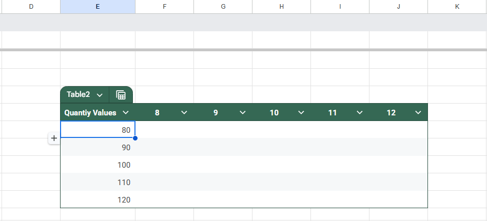
➤ Label horizontal row inputs in F5:J5 with different Price values.
➤ Label vertical column inputs in E6:E10 with different Quantity values.
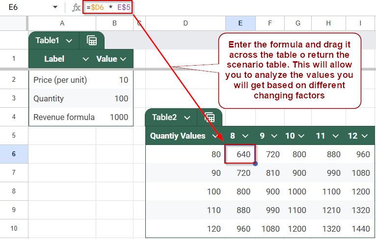
➤ In cell F6, enter the formula =$E6 * F$5 to calculate revenue using absolute references.
➤ Drag the formula across F6:J6, then down to F10:J10 to fill the full sensitivity table.
➤ Use the resulting table to analyze how revenue changes based on different price and quantity combinations.
What is Sensitivity Analysis in Google Sheets?
Sensitivity analysis in Google Sheets is a method used to understand how changes in input variables affect the outcome of a formula or model. It’s used for financial forecasting, budgeting, pricing, and decision-making models where you want to evaluate multiple “what-if” scenarios.
Instead of testing one value at a time, sensitivity analysis helps you observe how different combinations of inputs (like cost, price, or quantity) impact results like profit, revenue, or break-even points. In Google Sheets, this can be done using formulas, data tables, or drop-down-driven scenario setups.
Use a Sensitivity Table to Compare Scenarios
A sensitivity table is a simple and visual way to perform a sensitivity analysis in Google Sheets. It lets you test how changes in two variables, such as price and quantity, impact an output like revenue or profit. By laying out these variables across rows and columns, you can observe how different combinations affect your results. This method is ideal for financial modeling, pricing analysis, or business forecasting.
Steps:
➤ Set up your base formula. In a separate cell, calculate the base output. For example, in cell B4, enter:
=B2 * B3
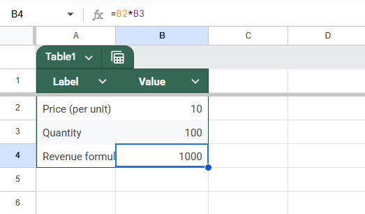
Where B2 is the Price (e.g., 10), and B3 = Quantity (e.g., 100), this formula calculates revenue as Price × Quantity.
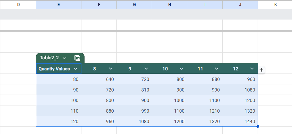
➤ Label your table inputs. Create your sensitivity table starting in E5. In cells F5:J5, enter different Price values horizontally (e.g., 8, 9, 10, 11, 12). In cells E6:E10, enter different Quantity values vertically (e.g., 80, 90, 100, 110, 120)
➤ Enter the sensitivity formula In the top-left cell of your data table (F6), enter this formula to calculate revenue for each combination:
=$E6 * F$5
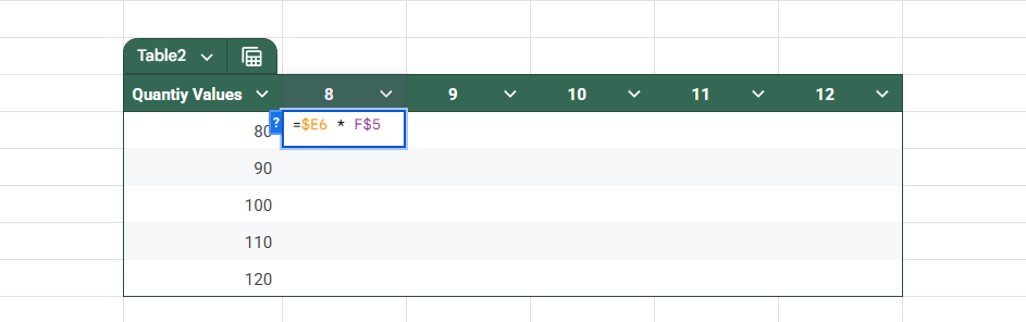
This formula multiplies the quantity from column E by the price from row 5, using absolute references to keep the right rows and columns fixed as you fill the table.
➤ Fill the sensitivity table. Drag the formula from F6 across to J6. Then drag the entire row F6:J6 down to row 10 (F10:J10)
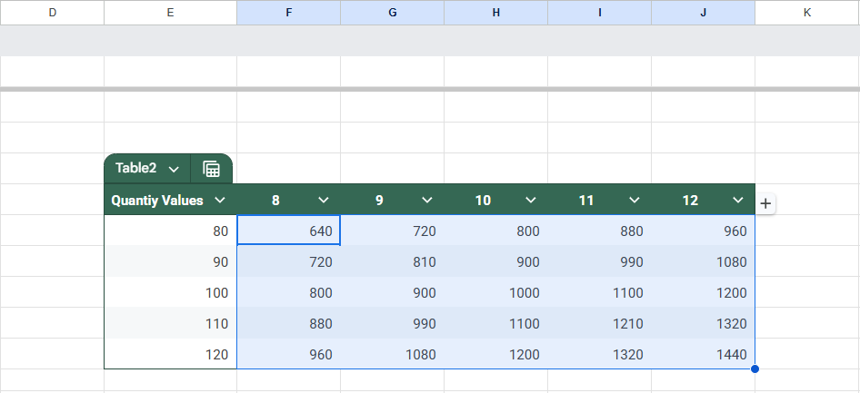
This fills your table with revenue values for all combinations of quantity and price.
➤ Analyze the results. Review the filled table to see how changes in quantity and price affect revenue. This allows you to quickly compare multiple scenarios side-by-side.
Utilize IF Statements to Model Threshold-Based Results
A practical way to run a sensitivity analysis in Google Sheets is by using IF statements to model how outcomes change when specific thresholds are met. This is especially helpful when dealing with conditions like bonus payouts, pricing tiers, or cost adjustments that only activate once certain limits are crossed.
By setting up =IF() formulas tied to variable inputs, you can quickly see how changes to your data influence the result. This method allows you to test and compare conditional outcomes efficiently.
Steps:
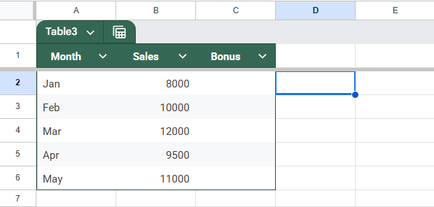
➤ Set up your input data, such as total sales in a cell (e.g., B2) that you want to test for thresholds.
➤ Write an IF formula based on the logic you’re modeling. For example, enter the formula in C2:
=IF(B2 > 10000, 1000, 0)
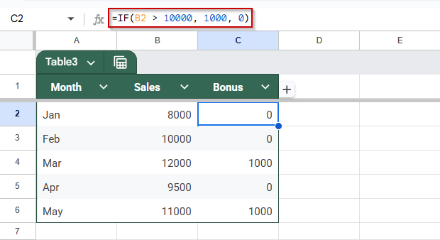
This means that if sales in B2 exceed 10,000, the bonus is $1,000; otherwise, it’s $0.
➤ Adjust the input value in B2 manually to simulate different scenarios (e.g., test sales values of 8000, 10000, 12000) and observe how the bonus changes.
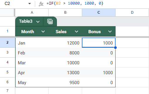
➤ Use this setup across a range if you want to apply the model to different thresholds, time periods, or products by dragging the formula down or across your sheet.
This approach helps you analyze how results respond to variable changes, especially when those changes trigger specific actions.
Create Dynamic Charts for Visual Sensitivity
Once you’ve built a sensitivity table with changing variables (like price and quantity) and resulting outputs (like profit), visualizing the data with a dynamic chart makes it easier to identify patterns, trends, and key turning points. This method helps you transform raw data into actionable insights, making it useful for reporting and presentations.
We will use the same sensitivity table that we had setup in the first method.
Steps:
➤ Select your entire sensitivity table, including the row headers and column headers, along with the calculated output values.
➤ Click on Insert in the top menu, then choose Chart.
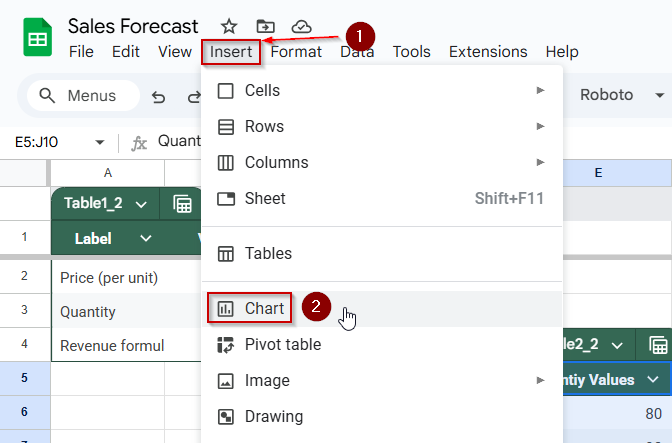
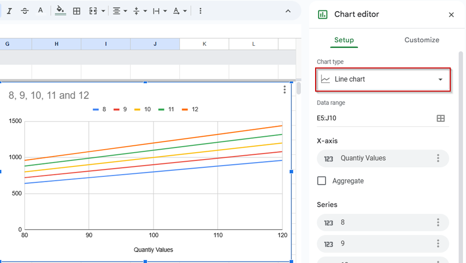
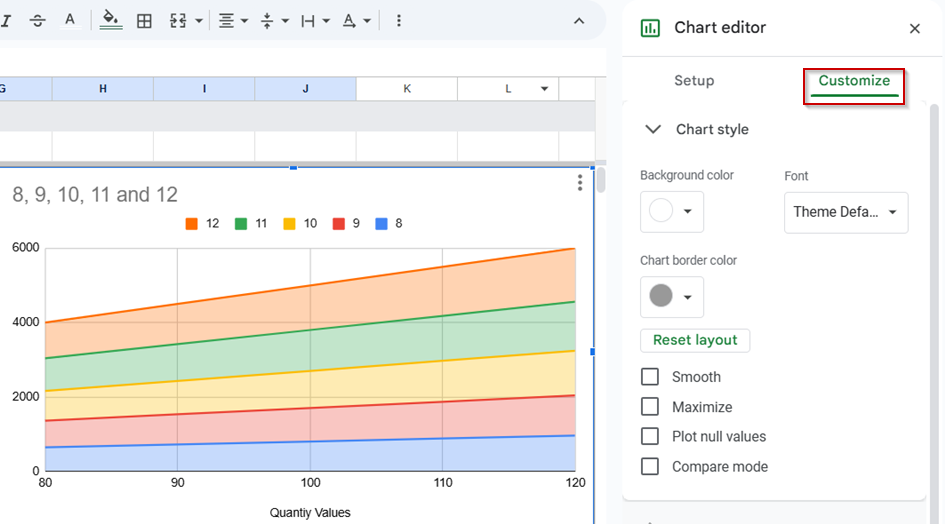
➤ Google Sheets will insert a default chart. In the Chart Editor panel on the right, change the Chart Type to:
- Line chart if you want to show trends across one variable (like how revenue changes with quantity for each price).
- Or an Area chart if you want to emphasize growth patterns.
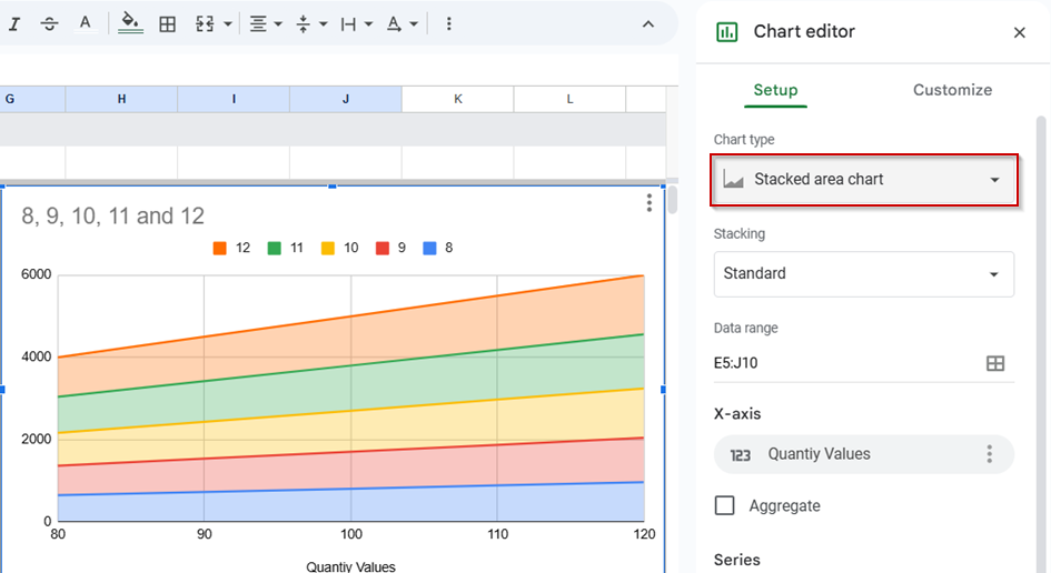
➤ Use the Chart Editor’s “Customize” tab to format however you like.
➤ Now, if your price or quantity inputs are cell-referenced (e.g., from named inputs or drop-downs), the chart will update automatically when those values change.
Employ Data Validation in Interactive Situations
One effective way to simulate sensitivity analysis in Google Sheets is by using drop-down menus through Data Validation. This method lets you switch between different input values, such as price points, growth rates, or cost assumptions, without manually editing cells each time. It keeps your model clean and user-friendly, making it ideal for dashboards or presentations that require real-time scenario testing.
Steps:
➤ Create a list of possible input values in a separate column or sheet (e.g., price options like 50, 60, 70, 80). Keep these values organized and labeled for clarity.
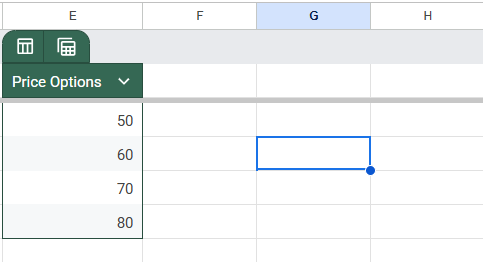
➤ Select the input cell where you want users to choose a variable (e.g., a cell labeled “Select Price”).
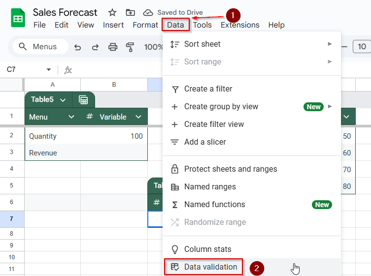
➤ Go to Data >> Data validation >> Drop-down. Choose “Drop-down” and select the cell range containing your input options. Click “Done” to apply.
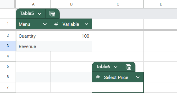
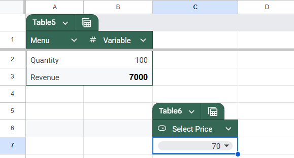
➤ Reference the drop-down cell in your calculations using standard formulas. For example:
=B2 * C7
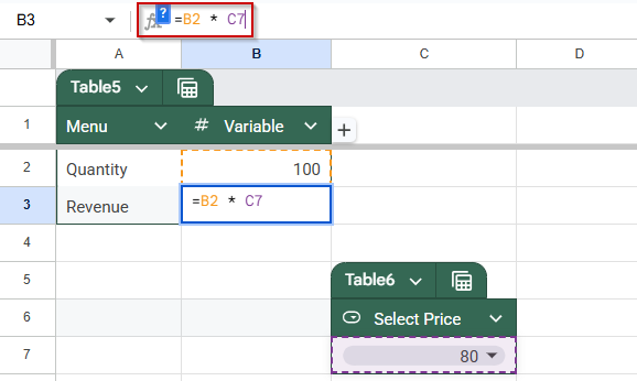
Where C7 is the drop-down with price, and B2 is the quantity.
➤ Test the interaction by selecting different values from the drop-down. Your linked formulas will instantly update based on the selection, allowing for real-time what-if exploration.
This technique enhances the interactivity of your sensitivity models, allowing for rapid, accurate, and visually clear scenario changes.
Frequently Asked Questions
What is sensitivity analysis in Google Sheets?
It’s a technique that lets you test how changes in one or more input variables affect the outcome of your formulas or model.
Can I do two-variable sensitivity analysis in Google Sheets?
Yes, by building a two-way data table with input combinations and referencing a base formula to fill results dynamically.
Do I need add-ons to run sensitivity analysis?
No, Google Sheets supports it natively using formulas like IF, INDEX, and table setups. Add-ons are optional for automation.
How is sensitivity analysis different from what-if analysis?
What-if analysis focuses on individual scenario outcomes, while sensitivity analysis examines how sensitive the output is to input changes.
Wrapping Up
Sensitivity analysis in Google Sheets is a powerful way to test how different input values affect your results. Whether you use simple IF statements, two-way data tables, drop-down menus, or dynamic charts, each method helps you explore multiple scenarios and make better-informed decisions. These tools are especially useful for forecasting, budgeting, pricing models, and business planning. By building interactive and flexible models, you can easily identify which variables have the most impact and adjust your strategy accordingly.