Have you ever wondered about alternative methods of auto-filling data in Google Sheets?
The traditional drag-and-drop method can be pretty hectic when dealing with large amounts of data. So we have brought you several alternatives for auto-filling that are simple, quick, and easy. From beginner to expert, everyone will find their way here.
In this article, we will go through the steps in detail and show you all the possible ways to autofill in Google Sheets without dragging.
➤ The Keyboard Shortcut ( Ctrl + D) method is great for smaller data sizes that you can easily select. It doesn’t require much time, but you must follow a few steps.
➤ When your data size is too large, the ArrayFormula is your friend. It autofills all the data just by typing one simple formula: ArrayFormula (C2: C + 10).
➤ Google’s built-in auto-fill pop-up box is the easiest one for all kinds of data. However, you must accept the Suggested Autofill as soon as it appears.
➤ Google offers another built-in Fill Down feature to make things easier. Locate the feature, and you’re good to go.

Autofill Using the Keyboard Shortcut
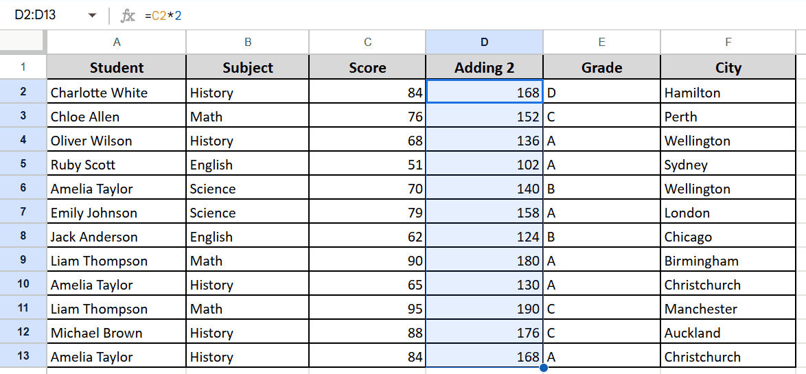
Using the keyboard shortcut is the easiest way to autofill data without dragging. For example, let’s say we want to multiply all the scores by 2. Here’s how you can do it:
Steps:
➤ Start by typing the formula in the first cell where you want the autofill to occur. Here, I want to autofill the D column, so I have typed the formula ‘=C2*2 ‘ in the first cell. Then hit Enter.
➤ Select the cell containing the formula (D2), hold down the Shift key, and select the last cell you want to fill (D13).
➤ Press Ctrl + D (for Windows) or Cmd + D (for Mac) to autofill the selected range.
Using ArrayFormula to Autofill Without Dragging
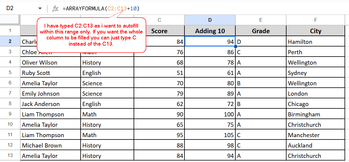
Using the ArrayFormula helps you autofill a whole column by typing the formula once. This is super easy and doesn’t require too many clicks. Let’s add 10 to all the scores in the C column for this method.
Steps:
➤ Like the previous method, select the first cell of the column you want to autofill (D2) and type the formula:
=ArrayFormula (C2: C + 10)
➤ That’s it! The whole column will be filled with new scores.
Autofill Using the ‘Suggested Autofill’ Box
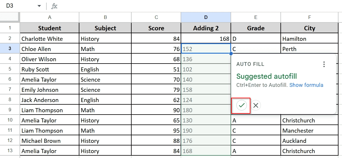
Google has a built-in Auto Fill option that pops up whenever you insert a formula in a cell. Here, you do not have to do anything; just insert the formula in the first cell of the column and hit the check button in the pop-up.
That’s all, the whole column will be auto-filled with data. Here, I have multiplied the scores by 2.
Using the Fill Down Feature
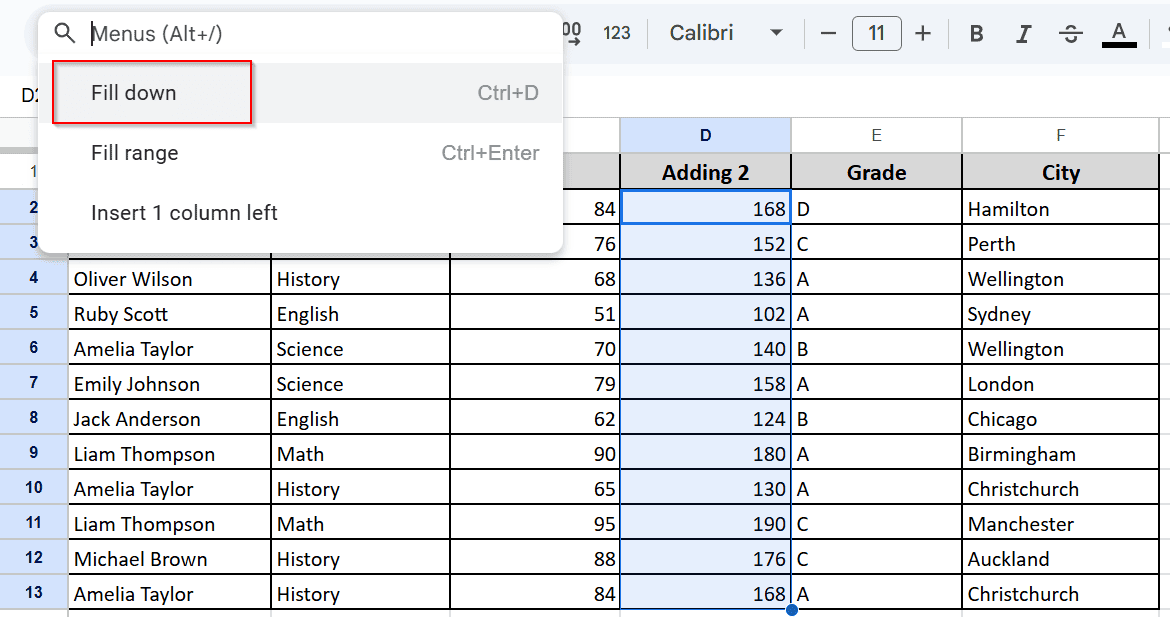
Google Sheets has a fill-down feature that completes the job in seconds. Enter the formula in the first cell of the column > Select the range > Search for Fill Down and Press.
Frequently Asked Questions
How do I stop Google Sheets from automatically filling numbers when dragging?
➤ Enter the value in a cell (25.5)
➤ Hold Ctrl (for Windows) or Cmd (for Mac) while dragging the fill handle.
This way, you will have the same number filled in the whole column.
Can I autofill text or words in Google Sheets?
Surely, you can.
➤ Type in the first text on the cell (e.g., Apple)
➤ Type the following text in the bottom cell (e.g., Banan)
➤ Drag it down, holding the small square in the bottom right, to the cell you want to fill.
➤ It will automatically fill the column with the pattern of text.
How do I undo autofill if it fills the wrong data?
To undo autofill: Press Ctrl + Z (for Windows) or Cmd + Z (for Mac) to undo the autofill action. This will revert the changes made by autofill.
Concluding Words
Auto-filling in Google Sheets doesn’t have to be limited to the traditional drag-and-drop method. We have discussed some quick and easy methods to save your efforts and time. No matter which method you choose, each of them will help you work more efficiently.
Master all the techniques with our easy guide. If you have any questions, let us know in the comments section. Also, don’t forget to let us know your opinion regarding the topic.