When you work in Google Sheets, the date format might not always match the region you need. This often happens when your spreadsheet is set to a different regional setting, and the dates show up in the US format instead of the UK format.
Adjusting the date format is a simple step that can make your data easier to read and more consistent with how dates are used in your location. It also helps avoid confusion, especially when sharing your spreadsheet with others or importing data from external sources.
In this article, you’ll learn how to change the date format to the UK style in Google Sheets using four easy methods.
One of the easiest and simplest methods to change date format to UK is using the TEXT function.
Here’s how you can apply this function:
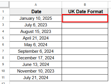
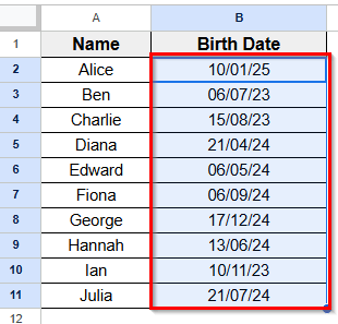
➤ Open your Google spreadsheet and create a table with Column A for the local date format and Column B for the UK date format result.
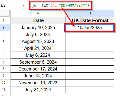
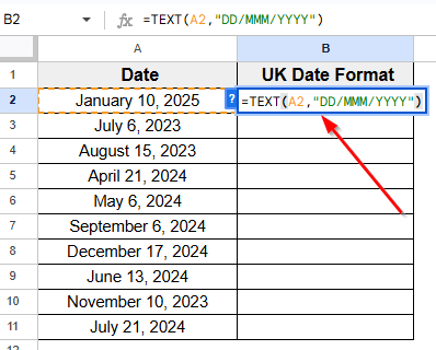
➤ Select cell B2, where we will enter the TEXT function to get the UK date format.
➤ Type the formula =TEXT(A2,”DD/MMM/YYYY”)
➤ Press Enter.
➤ You will now see the date in UK format. For example, January 10, 2025 to 10/Jan/2025.
What is Date Format in Google Sheets?
Date format in Google Sheets controls how a date appears in your spreadsheet. It sets the order of day, month, and year, like dd/mm/yyyy for the UK or mm/dd/yyyy for the US.
Google Sheets uses your spreadsheet’s regional setting to decide how dates should appear. It’s necessary to convert the date format to the correct one according to your needs to avoid confusion, especially when working with international data.
Changing Regional Setting To Apply UK Date Format
When you want to change date format in Google Sheets, this method will update the entire spreadsheet to follow the UK format. First, you have to change the regional setting to the United Kingdom so you can apply the date format from Google Sheets’ Format option.
Here’s a step-by-step guide to do that:
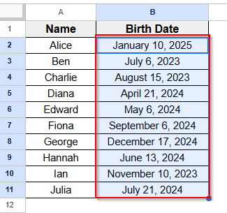
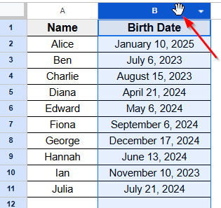
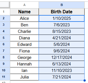
➤ Open your Google spreadsheet and create a table like the image below. For example, here we want to change the date format of Column B.
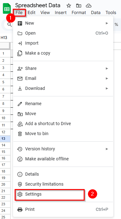
➤ Go to the top Menu and click on File option.
➤ Select Setting option from the dropdown menu.
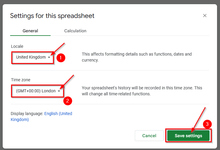
➤ A popup dialog box will appear where you can change the Locale region and Time zone.
➤ Now change the region to the United Kingdom and the Time zone to (GMT+00.00) London.
➤ Click on the Save Settings button. Google Sheets will now change the default date format to UK.
➤ Now your spreadsheet is ready to change the date format.
➤ Click on the Column B header to select the entire column.
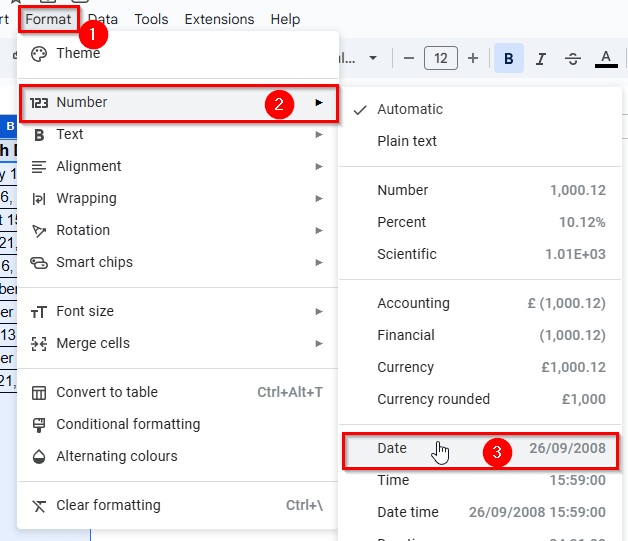
➤ Go to the top Menu and click on Format >> Number >> Date.
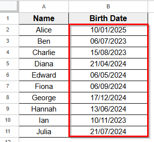
➤ Once you click on the Date option, you’ll see the date format of Column B converted to the UK date format. For example, January 10, 2025 becomes 10/01/2025.
Using The TEXT Function For Formatting
One of the easiest and simplest methods to change date format to UK is using the TEXT function.
Here’s how you can apply this function:
➤ Open your Google spreadsheet and create a table with Column A for the local date format and Column B for the UK date format result.
➤ Select cell B2, where we will enter the TEXT function to get the UK date format.
➤ Type the formula
=TEXT(A2,"DD/MMM/YYYY")
➤ Press Enter.
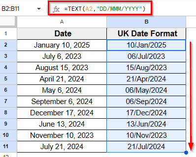
➤ You will now see the date in UK format. For example, January 10, 2025 to 10/Jan/2025.

➤ Now drag down the fill handle to copy the date format to the other rows in Column B automatically.
Using QUERY Function
This function is very helpful to change date format in Google Sheets, especially when working with large dataset. The QUERY function allows you to change the date format of the entire column at once.
Here’s how you can apply this formula:
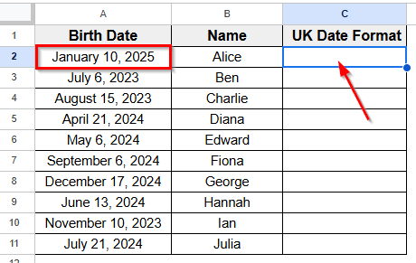
➤ Open your Google spreadsheet where the dates in Column A are in the local format. We want to use the QUERY function in Column C to display the entire Column A in UK date format.
➤ Select cell C2 which is right behind cell A2.
➤ Type the formula
=QUERY(A2:A11,"SELECT * FORMAT A 'DD/MMM/YYYY'").
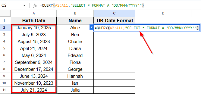
➤ Press Enter.
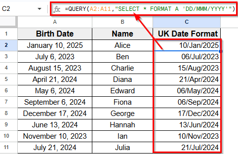
➤ You’ll see the UK date format appear in Column B, which is based on the dates from Column A.
Custom Date Format In Format Menu
You can also use Custom Date and Time to change date format local to UK.
Here’s the step-by-step guide to use this method:
➤ Select the range of cells in Column B.
➤ Go to the top Menu and click Format >> Number >> Custom Date and Time.
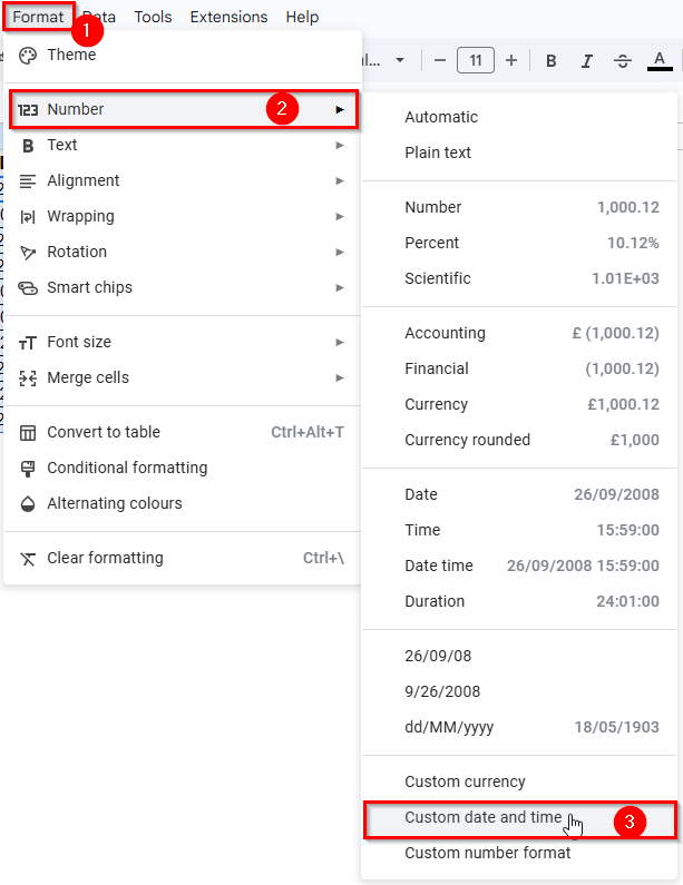
➤ A popup dialog box will appear that shows Custom date and time formats.
➤ Change it to the UK date format by selecting the date 05/08/30 (formatted as dd/mm/yy) in the list and click the Apply button.
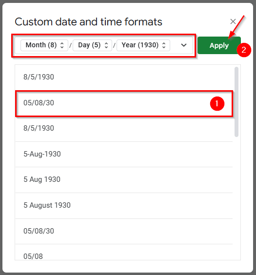
➤ Once you apply the format, you’ll see the date format of the selected cells are converted to the UK format.
Frequently Asked Questions
How do I change the date format to UK in Google Sheets?
To change the date format to the UK format (dd/mm/yyyy) follow the below steps:
➤ Select the column that has the value of the local date format.
➤ Go to Menu and click Format >> Number >> dd/MM/yyyy.
➤ Google Sheets change the date format of the selected cells or columns.
How do I convert US date format to UK date format in Google Sheets?
To change dates from US format (mm/dd/yyyy) to UK format (dd/mm/yyyy), follow these steps:
➤ Click on File in the top Menu.
➤ Select Settings.
➤ Change the Locale to the United Kingdom.
➤ Click Save and Reload.
➤ Go to Menu and click Format >> Number >> Date
Wrapping Up
Date format in Google Sheets controls how your dates show up, like if the day comes before the month or after. You might need to change the format to fit your location or make your data easier to read.
For example, the UK uses dd/mm/yyyy that is 10/Jan/2025, and the US uses mm/dd/yyyy which is Jan/10/2025. Changing the format helps keep your data clear and organized, especially when working with people in different places.
Sometimes, dates don’t change correctly if they aren’t recognized as dates. Using the functions we’ve applied in this article can help you to fix this problem quickly.

