
Our datasets in Google Sheets often contain sensitive or private information, and so, we need to hide them from certain users. To do this, you need to filter that information from the original dataset using FILTER, QUERY, or IMPORTRANGE and make a separate one.
This article will explain how you can use all of the FILTER, QUERY, and IMPORTRANGE functions to securely hide columns from certain users in Google Sheets.
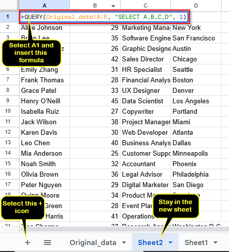
➤ Select the + icon on the bottom-left corner of your dataset and create a new sheet.
➤ Now, select cell A1 in the new sheet and insert this formula:
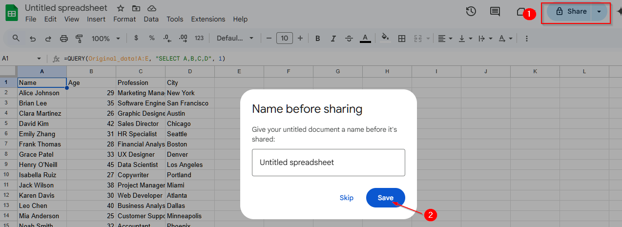
=QUERY(Original_data!A:E, “SELECT A, B, C, D”, 1).
It will return only the A, B, C, and D columns
➤ Finally, share the new dataset with other users.
Note: In the formula, replace “Original_data” with your own original dataset name and modify “SELECT A, B, C, D” with the columns you want to show.
Hide Columns in Google Sheets from Certain Users Using the QUERY Function
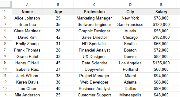
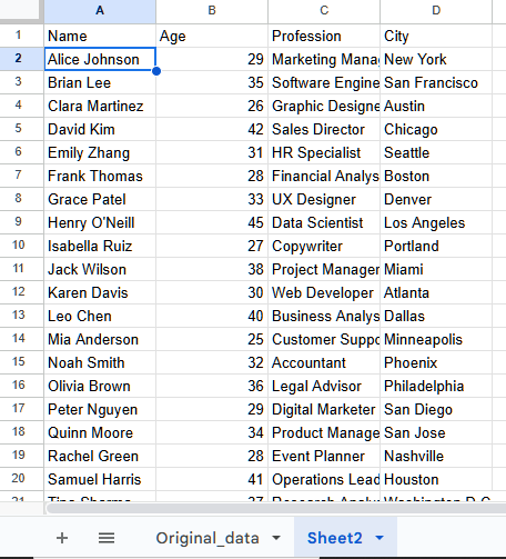
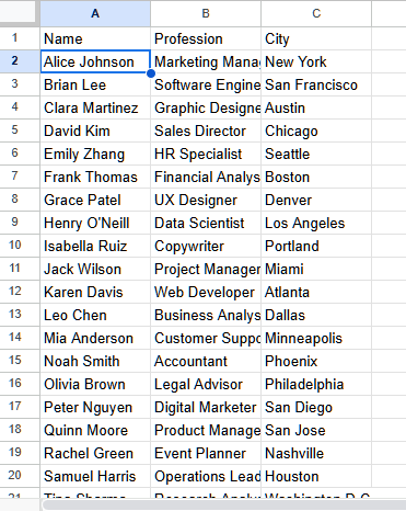
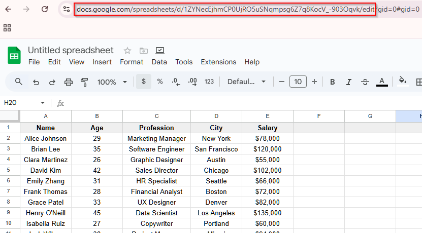
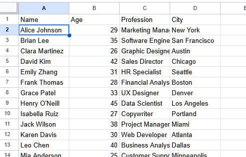
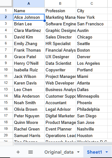
We have used the following dataset to demonstrate how to hide one or more columns in Google Sheets using the QUERY function. We will hide the “Salary” column first, and then both “Salary” and “Age” columns.
Hide One Column
Here is how to hide only one column using the QUERY function in Google Sheets.
Steps:
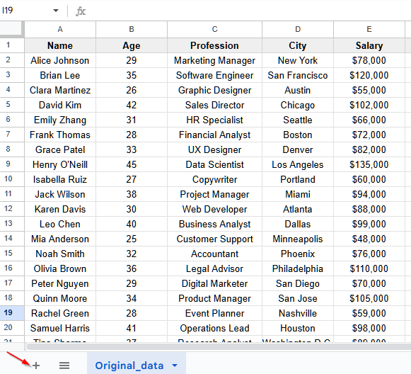
➤ Find the + sign at the bottom-left corner of your dataset and press it to create a new sheet.
➤ Now, select cell A1 in the new dataset and insert this formula:
=QUERY(Original_data!A:E, “SELECT A, B, C, D”, 1).
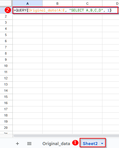
➤ Press Enter, and it will return the dataset without the “Salary” column.
➤ At the upper-right corner, look for the “Share” option and click on it.
➤ A pop-up window will be opened, and select the “Save” option.
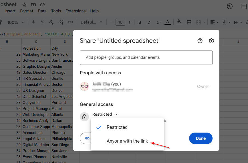
➤ Now, you will see an option named “Restricted”. Click on it, and press the option “Anyone with the link” if you want to share the dataset publicly.
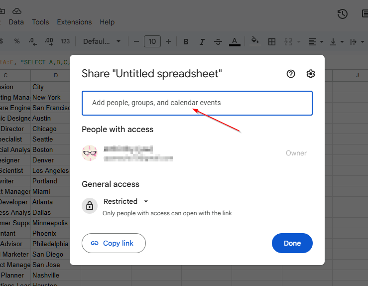
➤ If you want to share only with certain person (s), write down the email in the upper box and choose any role from editor, viewer, or commentor.
Hide Two Columns
We will hide the “Age” and “Salary” columns using the QUERY function in Google Sheets now.
Steps:
➤ Create a new sheet and select cell A1.
➤ Now, write down this formula:
=QUERY(Original_data!A:E, “SELECT A, C, D”, 1).
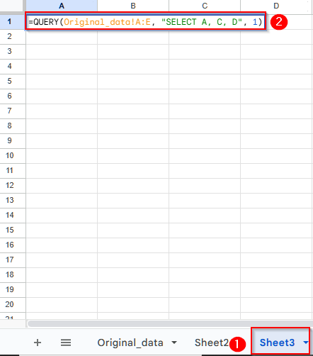
➤ Press Enter, and you will see the dataset without the columns “Age” and “Salary”.
➤ Now, share this new dataset with others, and they cannot see the “Age” and “Salary” columns.
Hide Columns in Google Sheets from Certain Users Using the IMPORTRANGE Function
IMPORTRANGE function imports a fixed range of the dataset and in the new dataset and hides columns from Google Sheets from certain users. However, it only works for a continuous range. If the range breaks, we will modify the IMPORTRANGE function using the QUERY function.
Hide Single Column
Here, I will use the IMPORTRANGE function to hide columns from certain users in Google Sheets.
Steps:
➤ Select the link of the original dataset till edit and press Ctrl + C to copy it.
➤ Create a new sheet and select cell A1.
➤ Now, insert the formula as:
=IMPORTRANGE(“https://docs.google.com/spreadsheets/d/1ZYNecEjhmCP0UjRO5uSNqmpsg6Z7q8KocV_-903Oqvk/edit”, “Original_data!A:D”).
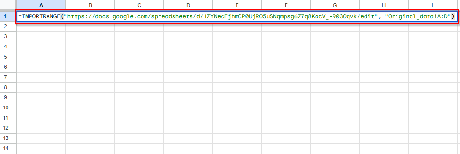
➤ Press Enter, and it will return the dataset without the column E, i.e., the “Salary” column.
Hide Non-Adjacent Columns
To hide non-adjacent columns (“Age” and “Salary”) using the IMPORTRANGE function, we will use a combined version of this function with the QUERY function.
Steps:
➤ Select the link of the original dataset till edit and press Ctrl + C to copy it.
➤ Open a new sheet and select cell A1.
➤ Insert this formula in that cell:
=QUERY(IMPORTRANGE(“https://docs.google.com/spreadsheets/d/1ZYNecEjhmCP0UjRO5uSNqmpsg6Z7q8KocV_-903Oqvk/edit”, “Original_data!A:E”), “SELECT Col1, Col3, Col4”, 1)
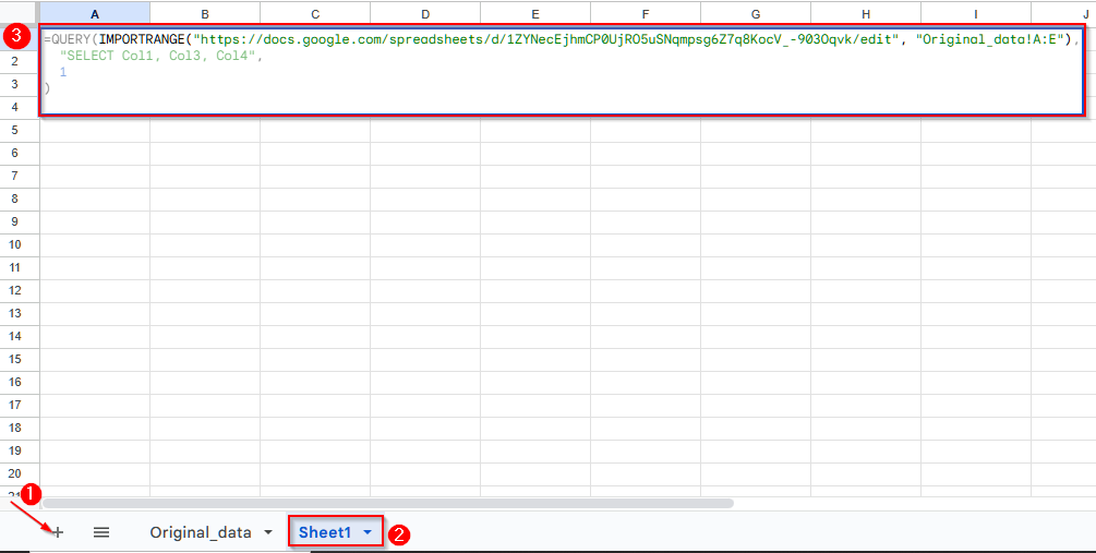
➤ Press Enter, and the dataset will return without the “Age” and “Salary” columns.

Hide Columns Using Filter Function in Google Sheets from Certain Users
Below, we will explain how you can hide one or more columns using the Filter function in Google Sheets from certain users.
Hide One Column
Here’s how to hide the “Salary” column using the Filter function in Google Sheets.
Steps:
➤ Open a new sheet and select cell A1.
➤ Now, insert the following formula:
=FILTER(Original_data!A:E, {TRUE, TRUE, TRUE, TRUE, FALSE})
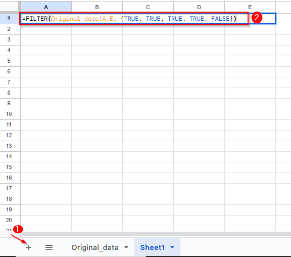
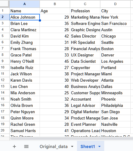
➤ Press Enter, and it will return the dataset without the “Salary” column.
Hide Multiple Columns
Below, we will use the Filter function to hide both “Age” and “Salary” columns from our dataset.
Steps:
➤ Create a new sheet and select cell A1.
➤ In the cell, insert the following formula:
=FILTER(Original_data!A:E, {TRUE, FALSE, TRUE, TRUE, FALSE})
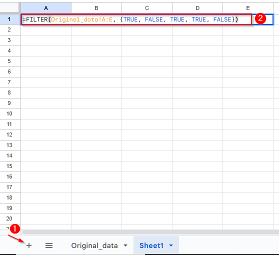
➤ Press Enter, and you will have a dataset without the “Age” and “Salary” columns.
Why Do You Need to Filter And Make a Separate Dataset?
Though you can hide certain columns and protect them in the original dataset from others, they can still view that data if they make a copy of the data or print it out. So, there is no way to completely hide certain columns from others in the original dataset. Thus, we need to filter the original to make a separate dataset.
FAQ
Can Viewers See Hidden and Protected Columns in Google Sheets?
No, viewers cannot unhide or see the hidden and protected columns in the same Google Sheets. However, in Google Sheets, there is no option to restrict anyone from copying a dataset. So, anyone can copy it and, after pasting it in a new sheet, they can view and edit that protected and hidden column.
Can I Hide Columns in Google Sheets Based on Users’ Roles?
There is no option to hide columns based on users’ roles, like editor, viewer, commenter, etc. However, you can use Google Apps Script to make a custom script and hide columns based on users’ roles.
Can I Use Conditional Formatting to Hide Columns in Google Sheets from Certain Users?
While conditional formatting is great at customizing the appearance of data, it cannot hide columns in Google Sheets. Similarly, other functions, like data validation, also cannot hide columns from certain users.
Wrapping Up
We have learned to use QUERY, IMPORTRANGE, and Filter functions to hide columns in Google Sheets from certain users in this article. Try these methods yourself and let us know if you have any inquiries.