
In the Google Sheets dataset, 0 (zero) often indicates missing data or invalid information. Thus, we need to ignore them when calculating the average to avoid getting inaccurate results. To exclude these zeroes from our average calculation, we can use AVERAGEIF, FILTER, ARRAYFORMULA, and QUERY functions.
This article will explain how to use these functions to calculate the average, ignoring zero (0) in Google Sheets.
➤ Select cell F1 and name it accordingly.
➤ Now, click on cell F2 and insert the following formula:
=AVERAGEIF(D2:D13, “<>0”)
➤ Click Enter on your keyboard, and it will return the average ignoring zeroes (0).
#Note: Replace the range part “D2:D13” with your desired column range. Like, if you want to calculate the average value of data in column C and this has 13 rows with row 1 being the header, then replace the range with “C2:C13”
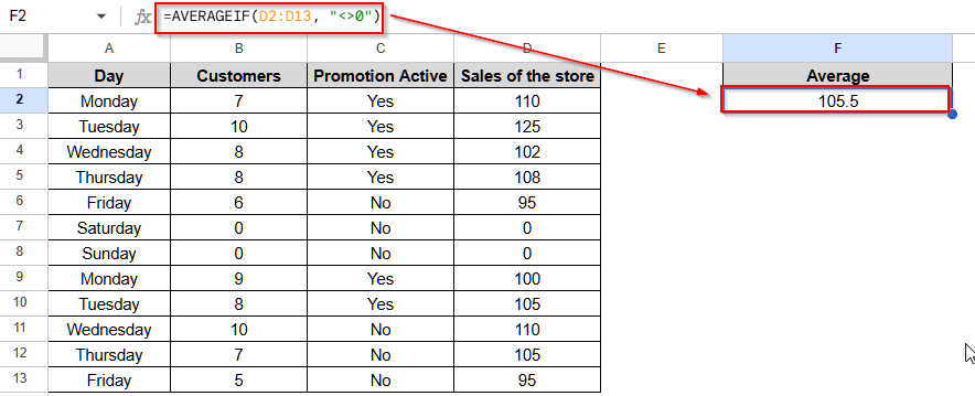
Calculate Average in Google Sheets Ignoring 0 (Zero) Using AVERAGEIF Function
The AVERAGEIF function allows the use of a condition that calculates the average, ignoring 0.
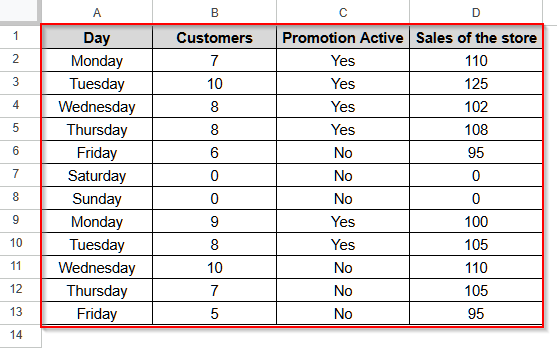
We will use the sales dataset of a store below to explain how to use the AVERAGEIF function in Google Sheets to calculate the average excluding zeroes. The store remains closed on Saturday and Sunday. So, the sales figure, zero, for these two days is not applicable to the store’s average sales.
Steps:
➤ Select cell F1 and name it “Average”.
➤ Now, select the cell F2 and insert the following formula:
=AVERAGEIF(D2:D13, “<>0”)
➤ Click Enter, and it will return the average of the sales of the store without considering the zeroes.

Using the FILTER Function
With a modified version of the Average function along with the Fillter function, you can calculate the average ignoring zeroes from a Google Sheets dataset.
Below, we have explained the method.
Steps:
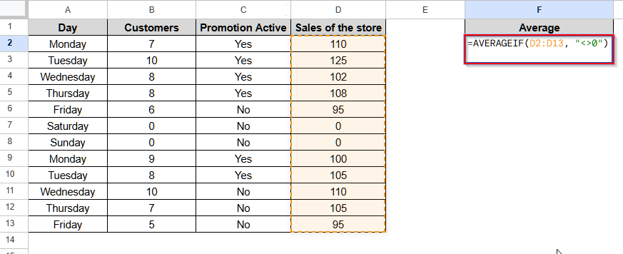
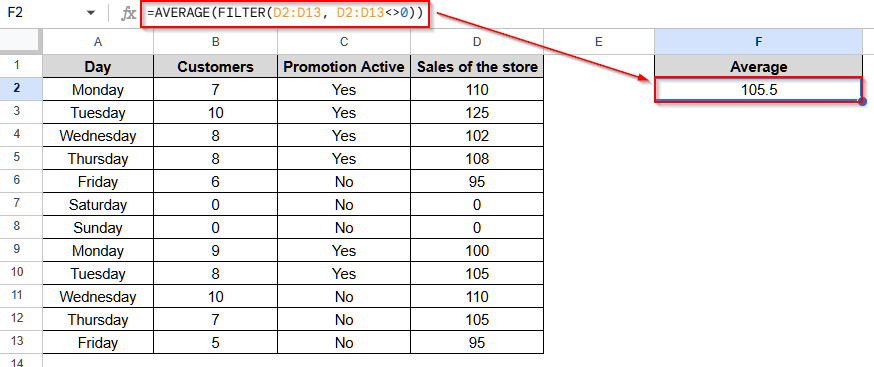
➤ Click on cell F1 and name it “Average”.
➤ Now, select the cell F2 and insert the following formula:
=AVERAGE(FILTER(D2:D13, D2:D13<>0))
➤ Finally, click Enter and the formula will return the average dales ignoring zeroes.
Note:
This modified AVERAGE formula is very flexible, and you can use multiple conditions here. Like, if you want to see the average of sales numbers above 100, use this formula:
=AVERAGE(FILTER(D2:D13, (D2:D13<>0)*(D2:D13>100)))
ARRAYFORMULA Function for Batch Calculation of Average Ignoring Zeros
ARRAYFORMULA is a versatile function in Google Sheets as it can process an entire range easily and so has multiple uses.
Below, we will explain the use of this ARRAYFORMULA to replace zeroes (0) with NA () and calculate the average ignoring 0 by combinning AVERAGE function with it.
Steps:
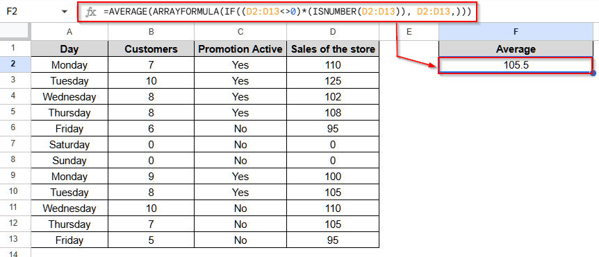
➤ Select cell F1 and name it “Average”.
➤ Then, select the cell F2 and insert the following formula:
=AVERAGE(ARRAYFORMULA(IF((D2:D13<>0)*(ISNUMBER(D2:D13)), D2:D13,)))
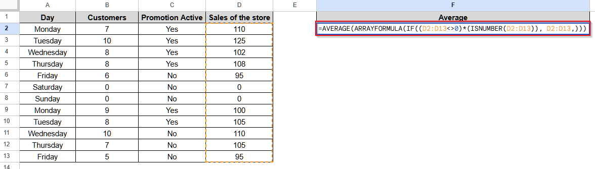
➤ Now, click Enter, and you will see the average without zeroes.
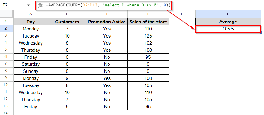
Using QUERY Function
Now, we will use the QUERY function to calculate the average in Google Sheets, ignoring zeros (0).
Steps:
➤ Select cell F1 and give it a name.
➤ Click on cell F2 and insert the following formula:
=AVERAGE(QUERY(D2:D13, “select D where D <> 0”, 0))
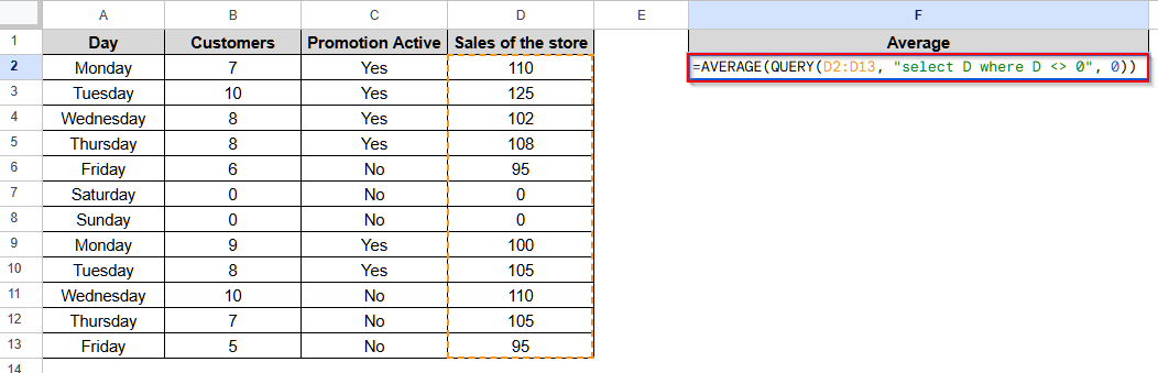
➤ Finally, press Enter on your keyboard, and you will see the returned average value excluding zeroes (0).
Frequently Asked Questions
Can I Calculate the Average of Some Non-Contiguous cells?
Yes, you can calculate the average of some non-contiguous cells using the AVERAGEIF function. Let’s say we want to calculate the average of the data in cells A1, A3, A5, and A7. Then, we will use the formula as: =AVERAGE(FILTER({A1, A3, A5, A7}, {A1, A3, A5, A7}<>0)).
How to Calculate Average If My Data Has #N/A Values?
To calculate data that has #N/A values, you will have to modify the condition in the AVERAGEIF function. Using the following formula, =AVERAGEIF(A1:A10, “<>#N/A”), you can easily do it. There, we replaced the condition, <>0 with <>#N/A.
Can I Calculate the Average of One Column Based on a Condition on Another Column, Ignoring Zeros (0)?
Yes, you can calculate the average for one column using a condition on another one using the AVERAGEIFS function. Suppose you have a product sales dataset, and column A is the category, column B is the sales amount. You want to calculate the average sales amount for “Category 1” products. For this, use the following formula: =AVERAGEIFS(B2:B10, A2:A10, “Category1”, B2:B10, “<>0”)
Wrapping Up
We have learned to use four different formulas to calculate the average in Google Sheets, ignoring 0 (zero) throughout this article. You can use all the functions, AVERAGEIF, FILTER, ARRAYFORMULA, and QUERY for any normal dataset. However, for a table dataset, it is better to use the QUERY function. Try these functions yourself and do not hesitate to reach out if you have any inquiries.