It’s common in Google Sheets to need data from one sheet while working in another. Instead of copying it yourself, you can link the cells. Then, when the data changes in the first sheet, it changes in the second sheet too.
This article uses simple formulas to explain how to reference a cell in another worksheet in Google Sheets. You’ll also learn how to reference a range of cells, create dynamic sheet references, and avoid common issues with cross-sheet linking.
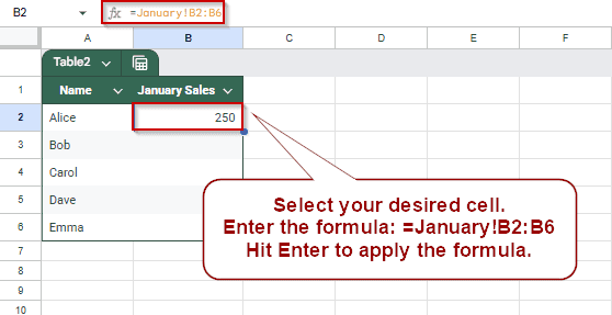
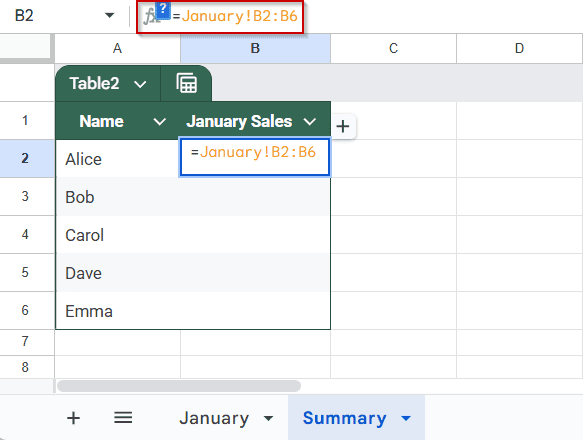
➤ Go to the destination sheet and select the starting cell (e.g., B2).
➤ Type the formula =January!B2:B6
➤ Press Enter.
➤ The selected range from the source sheet will appear in the destination sheet.
Reference a Single Cell from Another Sheet in Google Sheets
This method is useful when you need to import a specific value, such as a sales figure or total, from another worksheet into your current one.
In this example, the January sheet lists sales amounts for five team members. We’ll reference Alice’s sales, stored in cell B2, into the Summary sheet to centralize key data. Here’s how to link that cell directly.
Steps:
➤ Go to the Summary sheet where you want the referenced value to appear.
➤ Click on the destination cell (for example, cell B2) where you want to display the data.
➤ Type an equal sign (=) to start the formula.
➤ Click on the January tab to switch to the source sheet containing the data.
➤ Click cell B2.
➤ Press Enter.
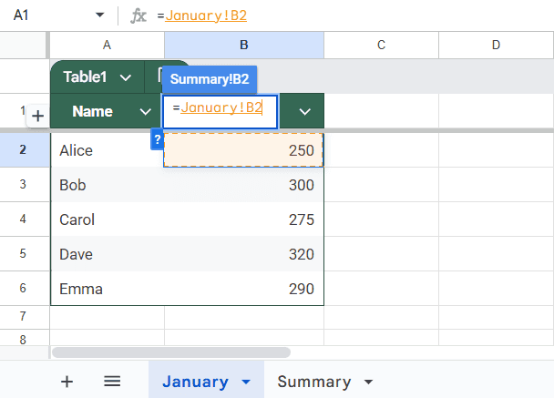
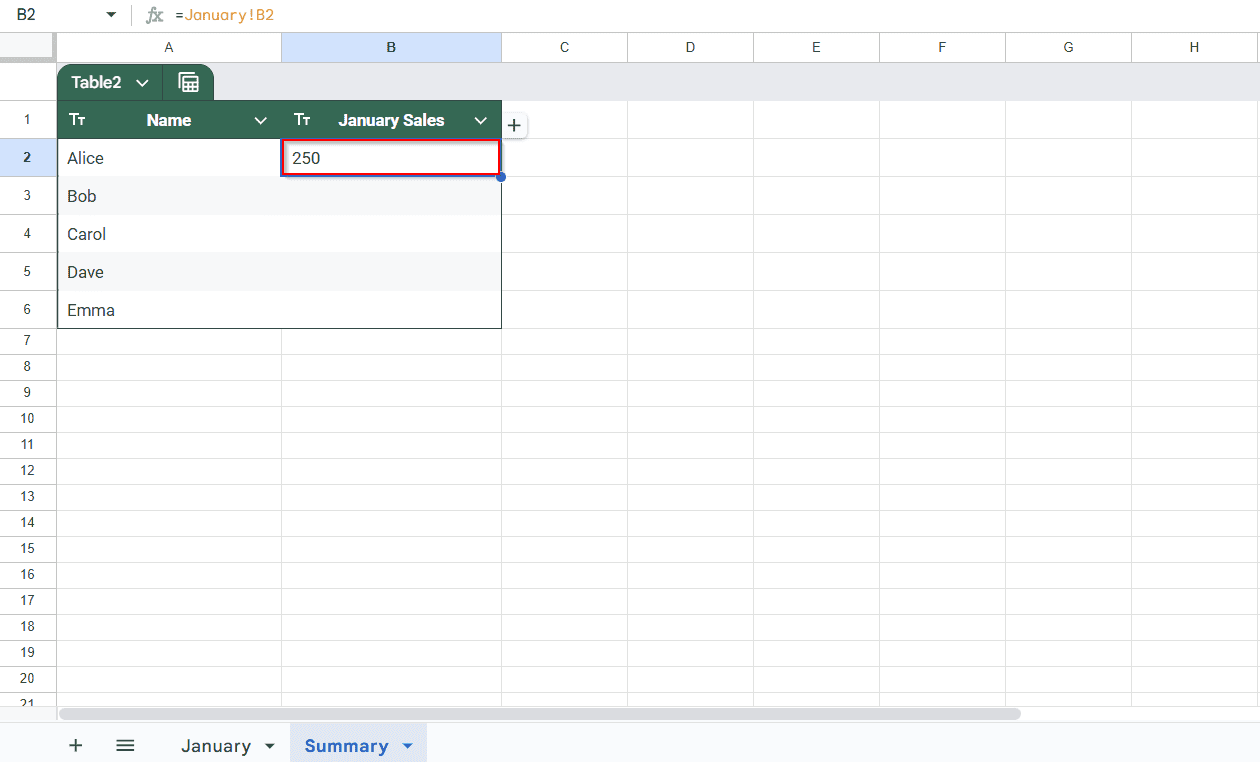
The formula =January!B2 will appear in the destination cell.
Reference a Cell Range from Another Sheet
You can also reference an entire range from another sheet. For example, to pull all sales values from the January sheet into the Summary sheet:
Steps:
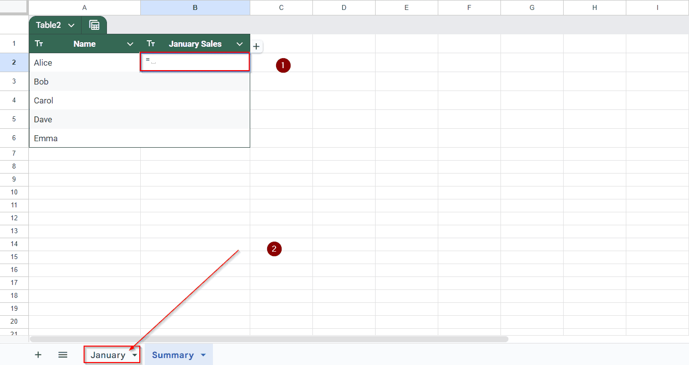
➤ Select the starting cell in the Summary sheet (e.g., B2).
➤ Type the formula
=January!B2:B6
➤ Press Enter.
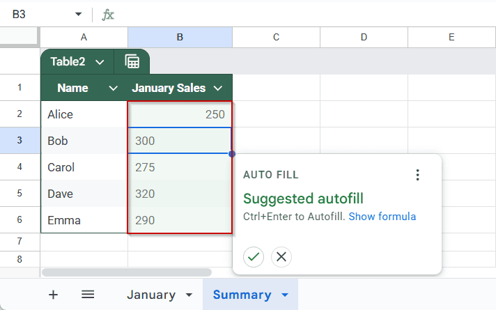
This will display the values from January!B2 to January!B6 in the Summary sheet.
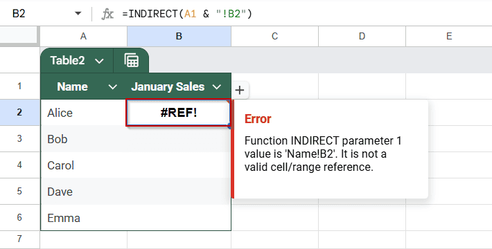
Create a Dynamic Reference Using INDIRECT Function
If someone types a sheet name, and you want to pull a cell from that sheet, you can do it without typing the sheet name yourself. Google Sheets lets you grab the info using the name the person entered.
Steps:
➤ In cell A1 of the Summary sheet, type the name of the source sheet (e.g., January).
➤ In cell B2, type the formula:
=INDIRECT(A1 & “!B2”)
The formula pulls data from cell B2 in the sheet named in A1.
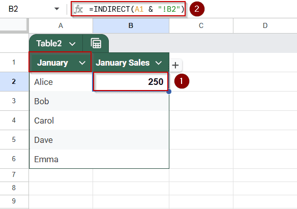
If A1 contains January, the formula evaluates to =January!B2.
Reference a Cell in a Sheet with Spaces in Its Name
If your sheet’s name has a space or something like a symbol, you’ve got to put single quotes around it in the formula. A lot of people miss that part, but if you leave out the quotes, Sheets won’t know what sheet you mean and will throw an error.
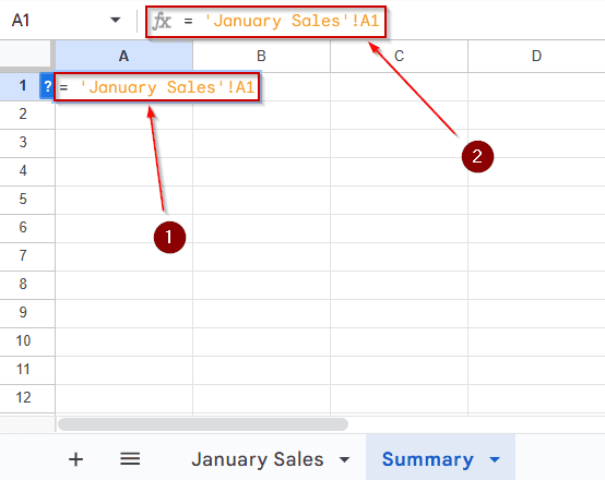
Let’s say your sheet is called January Sales, and you’re trying to get the value from cell A1. You’d write the formula like this: ‘January Sales’!A1. The quotes are important because of the space in the name.
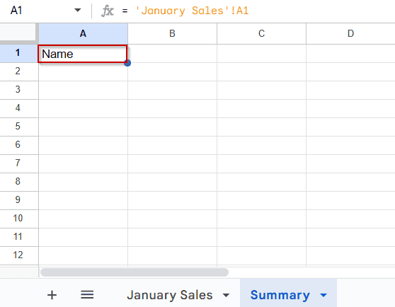
This tells Google Sheets to look for cell A1 in the January Sales sheet, even though the name includes a space.
Common Issues to Avoid When Referencing a Cell
Here are some common issues you might encounter while referencing cells across sheets:
➤ #REF! error: Occurs if the referenced sheet or cell doesn’t exist. Double-check the sheet name and cell reference.
➤ Case-sensitivity: Sheet names are not case-sensitive, but cell names are.
➤ Quotes: Always use single quotes for sheet names with spaces.
Frequently Asked Questions
Can I reference an entire column from another sheet?
Yes, you can. Just use a formula like =SheetName!B:B to pull all the values from column B in another sheet. It will also include anything new added to that column later.
What’s the fastest way to link two sheets?
The quickest method to link two sheets is:
➤ Type = in your destination cell
➤ Click the tab of the sheet you want to reference
➤ Click the cell you want to import the data from.
Google Sheets will automatically create the correct formula for you, linking both sheets instantly.
Can I reference a cell from a different spreadsheet?
Yes. Use the IMPORTRANGE function. The format is =IMPORTRANGE(“spreadsheet_url”, “Sheet1!A1”). This pulls data from another Google Sheets file, but you may need to grant access the first time.
How do I avoid broken references?
If you want to avoid broken references in your formulas, try not to delete or rename any sheets or cell ranges that your formulas are using. If you do need to make changes, like renaming a sheet or shifting things around, just make sure you go back and update any formulas that use those references. Otherwise, you’ll probably run into those annoying #REF! errors.
What happens if the referenced sheet is deleted?
If the sheet you’re pulling data from gets deleted, the formulas that were linked to it will break and show #REF! errors instead. That just means Google Sheets can’t find the data anymore. To fix it, you’d either have to bring that sheet back or get rid of the broken reference.
Wrapping Up
Linking cells from another sheet in Google Sheets isn’t too hard once you try it a couple of times. Whether you’re pulling one value, a full column, or grabbing data from a different spreadsheet, these tricks can really help you keep everything connected. Give them a shot with your own data. It’s a great way to stay organized and save time from doing things manually.