If you have two shipment records and want to find out which Product IDs from the first shipment are missing in the second, this guide will walk you through several quick and easy methods to do it, right inside Google Sheets. This is useful for logistics teams, inventory tracking, order fulfillment reviews, or verifying delivery consistency.
In this article, we’ll show you multiple ways to compare two columns of Product IDs side by side and instantly flag or list missing items. You’ll learn how to use Google Sheets formulas like MATCH, IF, VLOOKUP, COUNTIF, and even conditional formatting, perfect for comparing records from two shipments within the same spreadsheet.
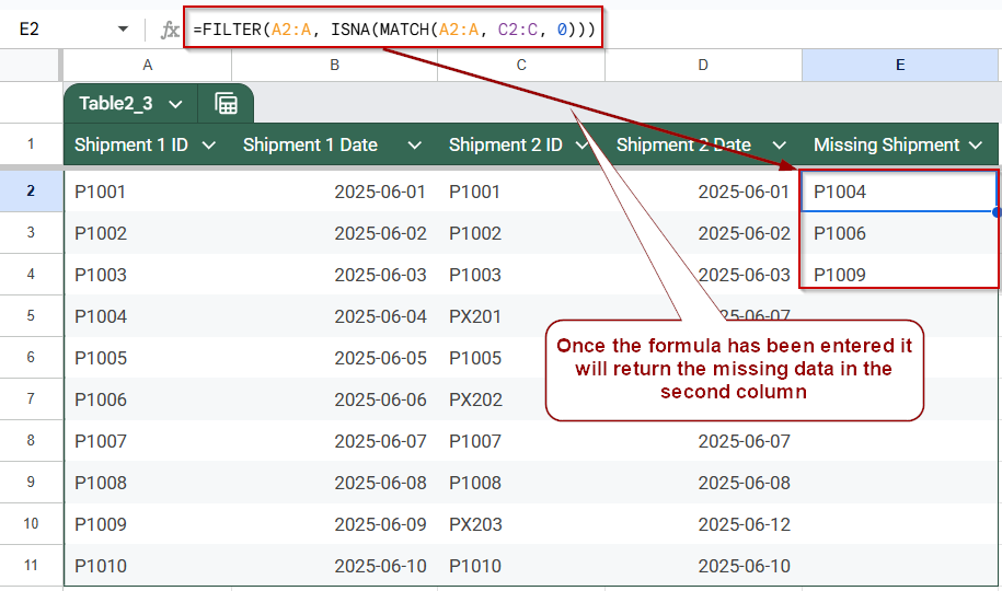
Steps to generate a clean list of missing Shipment IDs using FILTER + ISNA + MATCH:
➤ Go to a blank section of your sheet (e.g., Column E).
➤ In cell E2, enter this formula:
=FILTER(A2:A, ISNA(MATCH(A2:A, C2:C, 0)))
➤ Press Enter to display only the Shipment IDs missing from the attendance list.
➤ This method creates a clean, separate summary, ideal for reports, emails, or follow-ups.
Using MATCH & ISNA Functions to Find Missing Values
Using MATCH & ISNA to Find Missing Values in Google Sheets. This method uses the MATCH function combined with ISNA to identify values in one column that are missing from another, within the same sheet. It’s ideal for identifying Product IDs from the first shipment that don’t appear in the second shipment, allowing you to flag missing items instantly.
We’ll use a dataset that contains both columns: the Product IDs from Shipment 1 and Shipment 2.
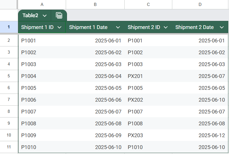
Both columns exist in the same sheet, side by side. This approach will add a helper column that automatically flags any Product ID from Shipment 1 as “Missing” if it’s not found in the Shipment 2 column.
Steps:
➤ Stay on your current sheet that contains both columns.
➤ In a new column (e.g., Column E), add the header ‘Missing Shipment’.
➤ In cell E2, enter the following formula:
=IF(ISNA(MATCH(A2, C:C, 0)), “Missing”, “”)
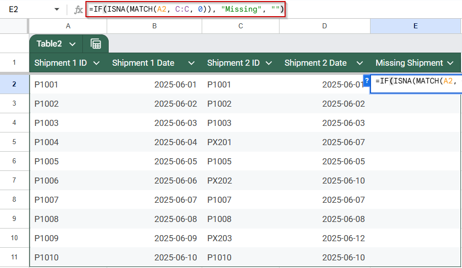
➧ C:C is the full column containing the Product IDs from Shipment 2.
➧ MATCH tries to find an exact match for the Product ID in the second shipment list. If not found, it returns an error.
➧ ISNA(...) detects this error.
➧ The IF function returns "Missing" if no match is found, or leaves the cell blank if the Product ID is present in Shipment 2.
➤ Drag the formula down to apply it to all rows in your Shipment 1 list.
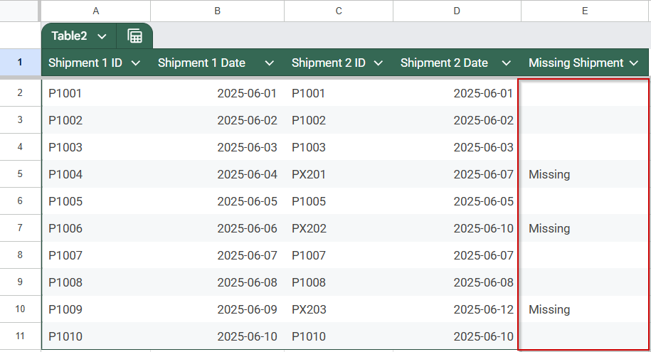
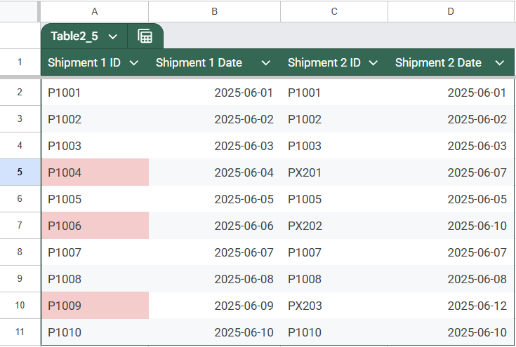
As you can see, the Status column gives the ‘Missing’ label based on the Product ID in column A. For example, IDs like P1004 and P1006 will be marked as “Missing” if they were replaced with PX-series codes in Shipment 2.
Flag Missing Entries with IF, ISERROR, and MATCH Functions
This method uses a simple combination of IF, ISERROR, and MATCH to identify Product IDs in your first shipment list that don’t appear in the second shipment. It’s especially helpful when both lists are in the same sheet, like in our example, and you want to flag missing data without returning errors.
Instead of cluttering your sheet with #N/A or raw error messages, this formula will insert a clean, readable label like “Not found” next to products that weren’t shipped the second time. The output is easy to interpret and ready for reporting, filtering, or follow-up.
This approach is ideal for warehouse teams or managers who need a quick visual cue showing which products weren’t included in a later shipment, without going through both lists manually.
Steps:
➤ Stay in your working sheet where both Product ID columns exist.
➤ In a new column (e.g., Column E), label it Missing Shipment.
➤ In cell E2, enter the following formula:
=IF(ISERROR(MATCH(A2, C:C, 0)), “Not found”, “”)
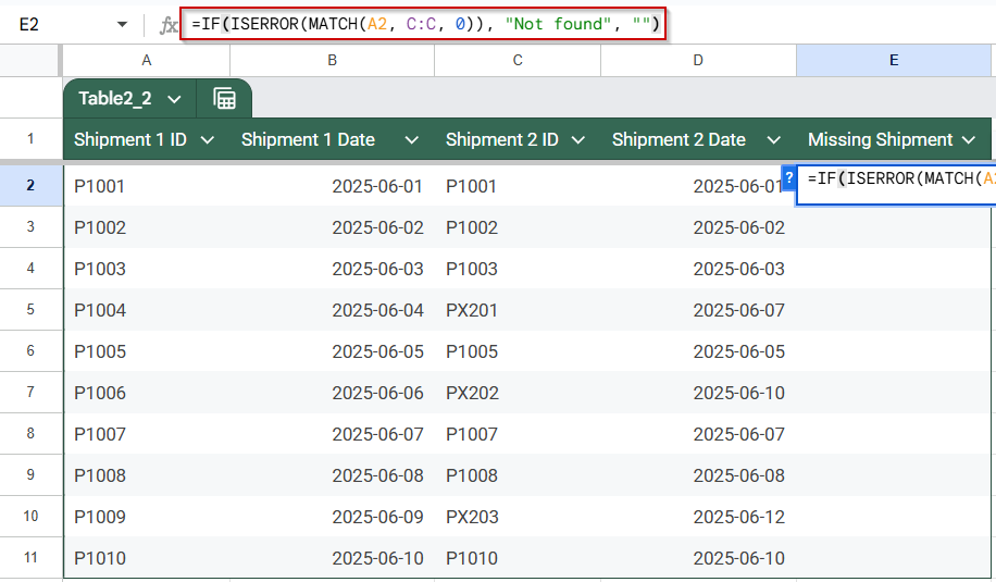
➧ MATCH(A2, C:C, 0) searches for that ID in the Shipment 2 column (Column C).
➧ If a match isn’t found, it returns an error.
➧ ISERROR(...) captures the error.
➧ IF(...) returns "Not found" if the ID is missing, or an empty cell if it is present.
➤ Press Enter and drag the formula down to apply it across all rows.
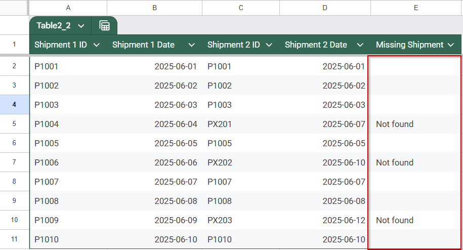
As shown in the Status column, the formula flags rows as “Not found” based on whether the Product ID in column A appears in the second shipment. For instance, Product IDs like P1004 and P1006 will be marked as missing because they are replaced by PX201 and PX202 in the Shipment 2 column.
Generate a Clean List of Missing Entries Using FILTER, ISNA, and MATCH Functions
If you need a quick, clutter‑free list of all products that shipped the first time but didn’t appear in the second shipment, this method is ideal. By combining FILTER, ISNA, and MATCH, you can return only the Product IDs that are missing from the second‑shipment column, without adding extra status columns.
Unlike earlier approaches that tag every row, this technique produces a separate, clean summary, perfect for emails, follow‑ups, or final reconciliation reports. It skips over items that did ship in both rounds and shows only the IDs that require attention.
Steps:
➤ Go to a blank section of your sheet (e.g., Column E).
➤ In cell E2, enter the following formula:
=FILTER(A2:A, ISNA(MATCH(A2:A, C2:C, 0)))
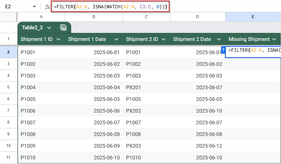
➧ If a Product ID is not found, MATCH returns #N/A.
➧ ISNA(...) detects these missing matches.
➧ FILTER(...) then returns only those IDs from Column A that are missing from Column C.
➤ Press Enter and let Google Sheets display the filtered results.
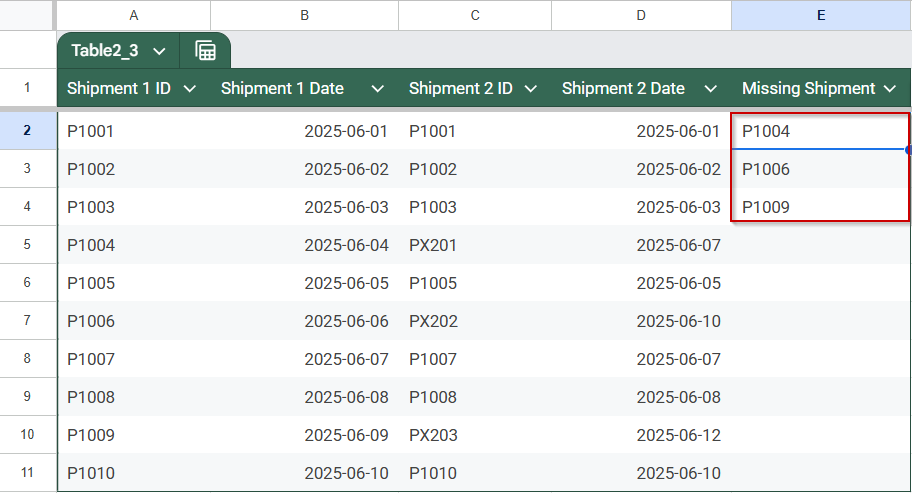
You’ll get a separate list showing only the Product IDs that are absent from the second shipment, no labels, no blanks, just the items that need follow‑up or investigation.
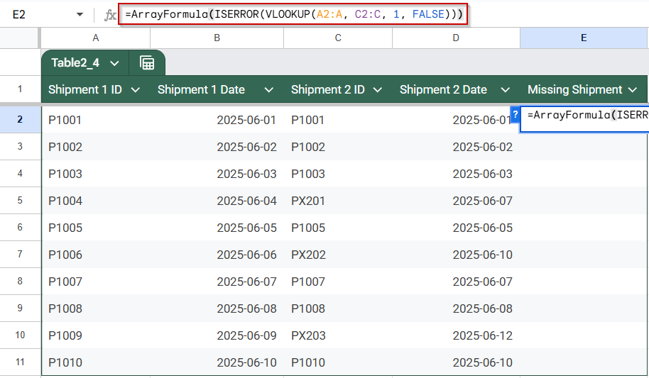
Detect Missing Items Using ArrayFormula, VLOOKUP, and ISERROR Functions
This method uses ArrayFormula with VLOOKUP and ISERROR to scan an entire list of Product IDs at once and flag which items from the first shipment are missing in the second. Unlike row-by-row formulas, this approach applies a dynamic formula that automatically fills the entire column, returning TRUE for missing items and FALSE for those that are found.
Steps:
➤ In your working sheet, create a new column next to the Shipment 1 data (e.g., Column E) and label it Missing in Shipment 2?
➤ In cell E2, enter the following formula:
=ArrayFormula(ISERROR(VLOOKUP(A2:A, C2:C, 1, FALSE)))
➧ If a Product ID is not found, VLOOKUP returns an error.
➧ ISERROR(...) flags these missing entries as TRUE.
➧ ArrayFormula(...) applies this logic across the full range in one step, no need to drag the formula.
➤ Press Enter, and the formula will instantly populate down the column.
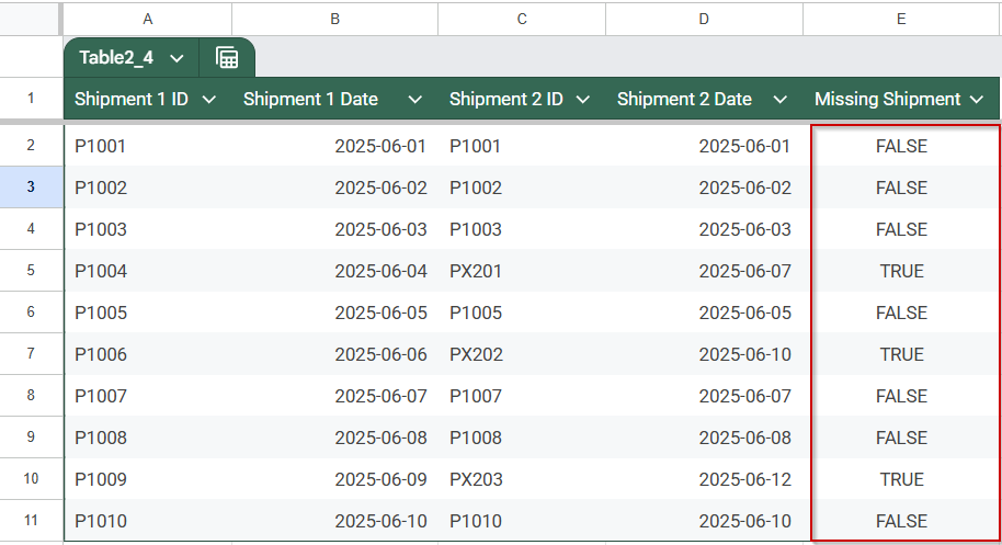
This solution is ideal when you want a quick and scalable TRUE/FALSE flag to identify missing entries across a large dataset, all in one go.
Highlight Missing Values Using Conditional Formatting Across Two Sheets
This method uses conditional formatting along with MATCH and ISNA to automatically highlight Product IDs from Shipment 1 that are not found in Shipment 2. Instead of adding helper columns or formulas in cells, this approach offers a real-time visual indicator for missing entries, ideal for quick reviews, audits, or error checks.
Whenever the data changes, the highlighting updates instantly, helping you stay on top of discrepancies between the two shipments.
Steps:
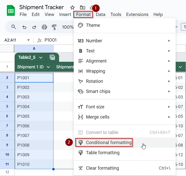
➤ In your working sheet, select the range of Product IDs from Shipment 1, e.g., A2:A11.
➤ Go to Format >> Conditional formatting.
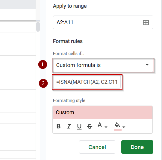
➤ Under Format rules, choose Custom formula is.
➤ Enter this formula:
=ISNA(MATCH(A2, C2:C, 0))
➧ If the ID isn’t found, it returns #N/A.
➧ ISNA(...) detects these missing entries and triggers the formatting.
➤ Choose a formatting style, such as a red background or bold text, to visually flag the missing IDs.
➤ Click Done.
Once applied, the cells in Column A will automatically highlight if their corresponding Product ID is not found in Shipment 2, no extra formulas or manual checks required.
Frequently Asked Questions
How can I find just the missing values between two columns?
Use this formula to find missing values between two columns:
=FILTER(A2:A, ISNA(MATCH(A2:A, C2:C, 0)))
This returns only the items found in your master list, but not in the attendance column.
Can I compare two columns without causing errors (#N/A)?
Yes, wrap your lookup in ISERROR or ISNA inside an IF. This flags missing values cleanly (e.g., “Not found”), rather than showing error codes.
What formula shows matching or non-matching IDs row by row?
Use =A2=D2 for TRUE (match) / FALSE (no match). Or extend with IF(A2=D2, “Match”,”No Match”) to get readable labels instead.
Can I highlight missing entries using conditional formatting?
Yes, select your master ID range and use a custom formula like =ISNA(MATCH(A2, D:D, 0)), then apply a fill color to flag any missing IDs.
How do I ignore blanks when comparing columns?
Wrap your formula in IF to skip empty cells. Example: =IF(A2=””,””,IF(ISNA(MATCH(A2,D:D,0)),”Missing”,””))
This ensures blanks aren’t flagged.
Wrapping Up
Comparing two columns to find missing values in Google Sheets doesn’t have to be a manual task. Whether you’re flagging attendance gaps, tracking records across sheets, or building summary reports, these formula-based methods make it fast and accurate. From simple IF statements to advanced filters and conditional formatting, you now have a range of tools to match your workflow. Try each one and pick the approach that best fits your data and reporting needs.