Comparing dates in Google Sheets is essential when you are tracking deadlines and project timelines or scheduling events. Whether you are checking which date is earlier or later, Google Sheets makes it easy with simple formulas.
In this tutorial, you will learn step-by-step how to compare dates in Google Sheets using built-in formulas and conditional formatting.
➤ The IF function compares two dates and returns a custom result based on the condition.
➤ Use =IF(E2<TODAY(), “Overdue”, “Upcoming or Today”). This checks if the date in E2 is earlier than today and returns “overdue,” “upcoming,” or “today.”
➤ To apply this method, insert the formula in a new column and press Enter.
➤ It will return “Overdue” if the due date is earlier than today; otherwise, “Upcoming or Today.”

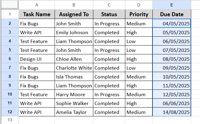
In this article, we will work with a task management dataset and apply methods like direct comparison, logical operators with TODAY & other functions, and conditional formatting. These techniques will help you determine which date is earlier or later, identify overdue tasks, and calculate how many days are left before a deadline.
Using Logical Operators to Compare Dates
You can use logical operators =, <, and > to directly compare dates in Google Sheets. These operators help identify if a task is due today, overdue, or upcoming by comparing each due date with the current date. This method is simple yet powerful for building condition-based outputs or filtering data dynamically.
Steps:
➤ Select an empty cell besides the due date column and name it Overdue?
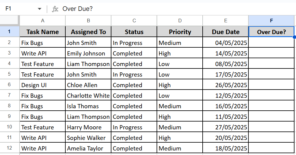
➤ Enter the following formula:
=E2>TODAY()
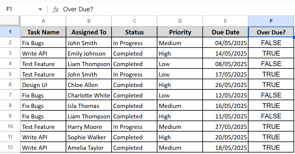
➤ Press Enter and drag to apply to all rows.
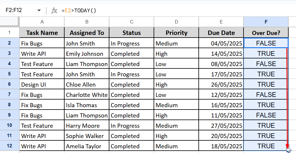
➤ It returns TRUE for overdue tasks and FALSE for those due today or later
Using IF Function For Custom Output
If you want to return a custom label based on each task’s due date, you can use the IF function. This allows you to achieve a specific output text like overdue, due today, or upcoming, depending on the current date. The formula compares the due date of each task with today’s date and returns a conditional result.
Steps:
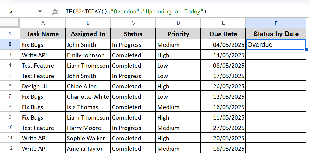
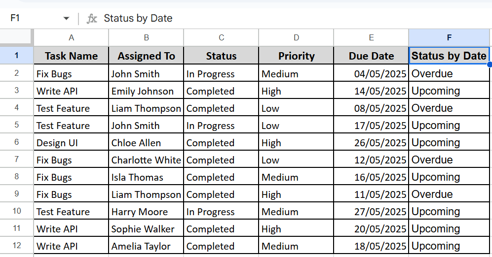
➤ Insert a new column to the right of the due date column and name it Status by Date.
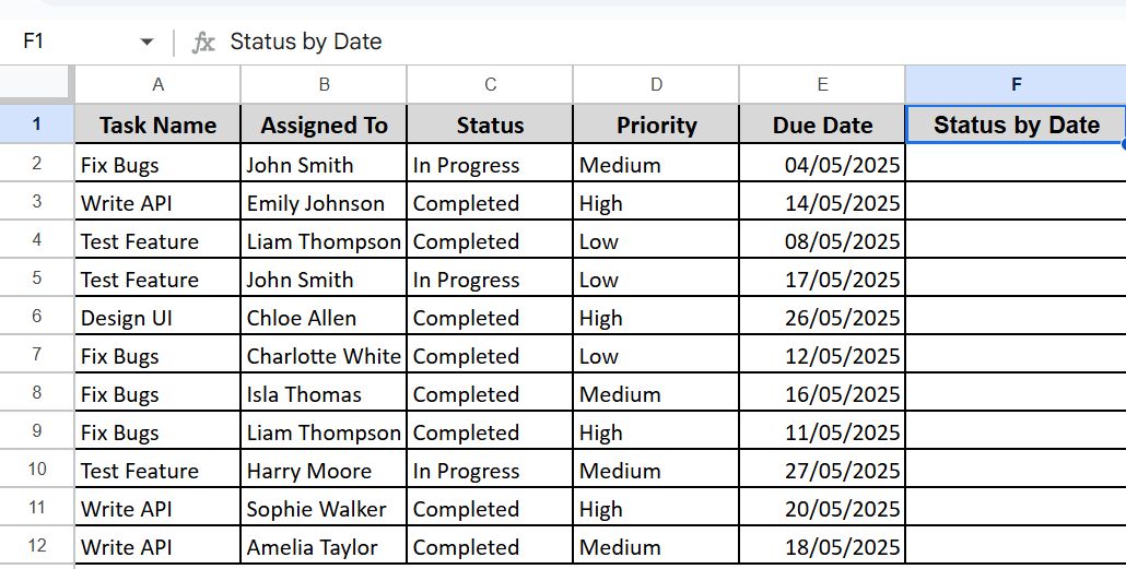
➤ In the first cell under new column (F2), enter the formula
=IF(E2<TODAY(),”Overdue”,”Upcoming or Today”)
➤ Press Enter.
➤ Drag the fill handle down to apply the formula to all rows (F2 to F12)
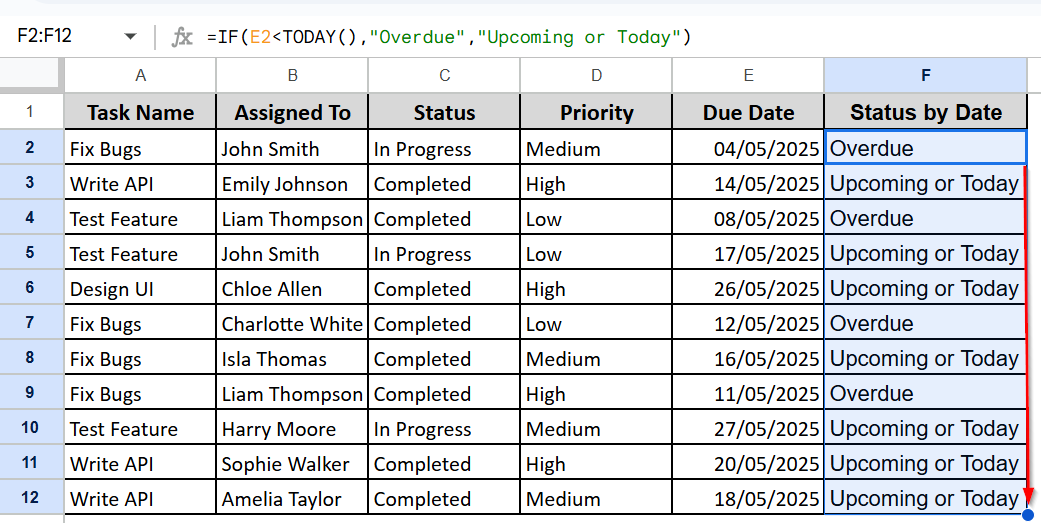
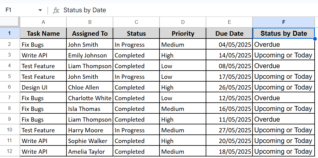
➤ The formula will return “Overdue” if the due date is earlier than today’s date; otherwise, it will return “Upcoming or Today.”
Using TODAY to Track Live Deadlines
If you want your task deadlines to update automatically based on the current date, you can use the TODAY function. This function returns the current date and updates every day you open the sheet. By combining it with logical formulas, you can easily monitor which tasks are overdue, due today , or upcoming. You don’t have to input any manual updates.
Steps:
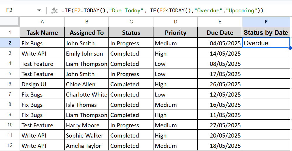
➤ Insert a new column to the right of the Due Date column and name it Status by Date.
➤ Enter the Formula in F2
=IF(E2=TODAY(),”Due Today”, IF(E2<TODAY(),”Overdue”,”Upcoming”))
➤ Press Enter.
➤ Drag the fill handle down to apply the formula to all rows (F2 to F12)
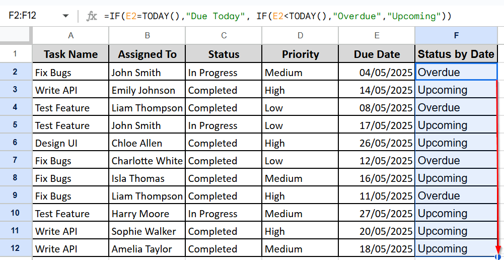
➤ It will return Overdue, Upcoming, or Due Today depending on the current date and each task’s due date.
Using Conditional Formatting for Visual Outcome
To make your task list more intuitive, apply conditional formatting to highlight deadlines with different colors. This feature lets you visually identify overdue, due today, and upcoming tasks by using simple date-based rules on the Due Date column. We are going to highlight the due date in red if the task is overdue and the due date in yellow if the task is due today and not yet completed. The due date is in green for upcoming tasks that are due in the future and not completed.
Steps:
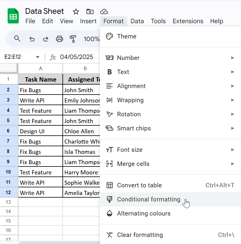
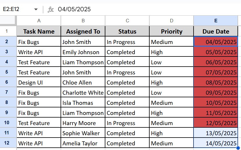
➤ Select the Due Date column and click and drag to select the Due Date cells (E2:E12)
➤ Go to Format >> Conditional Formatting
➤ Use a custom formula. In the Conditional format rules sidebar: Under “Format cells if,” choose “Custom formula is” and enter this formula:
=E2<TODAY()
➤ Set a red fill color to indicate the task is overdue.
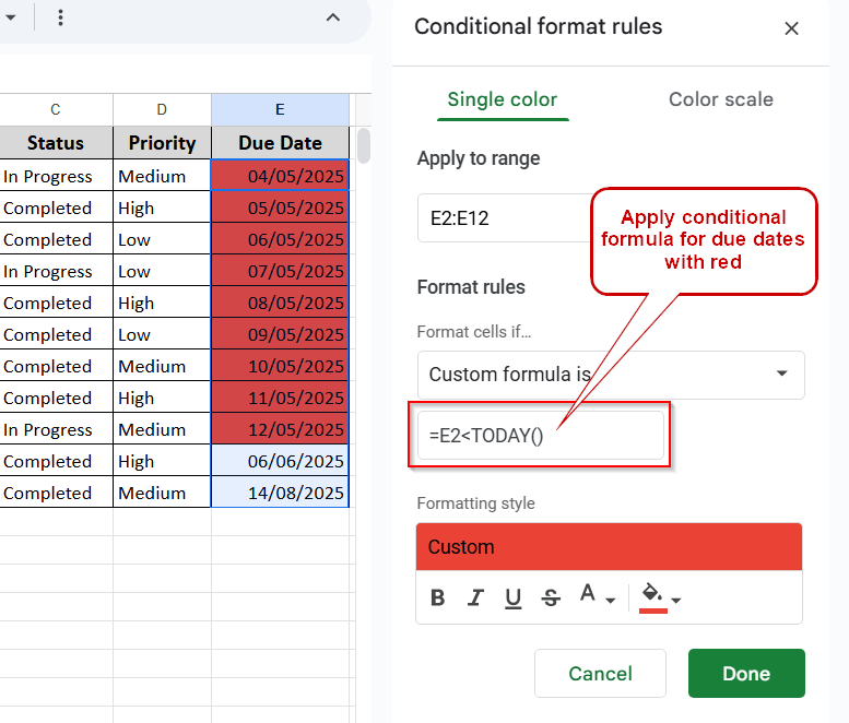
➤ Click Done.
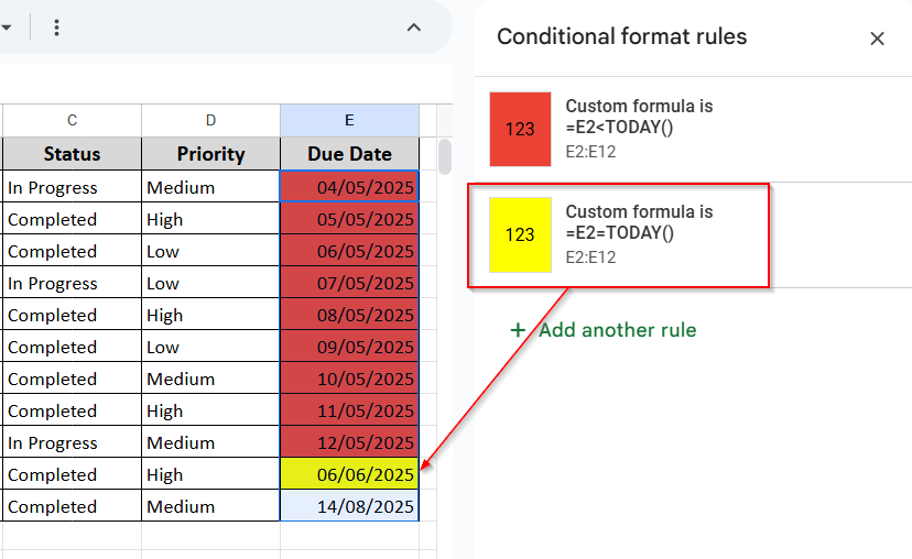
➤ Add another rule in the same way for due today and enter this formula:
=E2=TODAY()
➤ Set a yellow fill color to indicate the task is due today. It will return the color on the due date today.
➤ Add another rule in the same way for upcoming and enter this formula:
=E2>TODAY()
➤ Set a light green fill color to indicate the task is upcoming. It will return the color on the upcoming date.
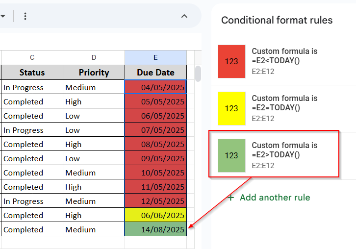
➤ It will return Overdue, Due Today, or Upcoming depending on the current date and each task’s due date, giving you visual cues for better task tracking.
Frequently Asked Questions
How do I check if two dates are equal in Google Sheets?
Use =A1=B1. It returns true if both dates are same
Can Google Sheets highlight overdue tasks automatically?
Yes. Use conditional formatting with =E2<TODAY().
Why is my date comparison not working?
Make sure your cells are formatted as dates, not plain text.
Can I calculate how many days are left until a task is due?
Yes. Use =E2-TODAY() or =DATEDIF(TODAY(), E2, “D”).
Wrapping Up
In this article we will learn how to compare dates in Google Sheets using logical operators and IF and TODAY() formulas and conditional formatting. These methods help monitor deadlines, flag overdue items, and maintain organized project tracking. Try applying these to your own spreadsheets to keep your tasks on schedule.