
We often need to check if there are any duplicates in the data in Google Sheets to avoid repeating the same information multiple times. For this purpose, we can use Conditional Formatting feature or functions like COUNTIF and FILTER. In this article, we’ll cover all of these suitable methods with a step by step guide.
➤ First, select cell E1 and write Duplicate as the name.
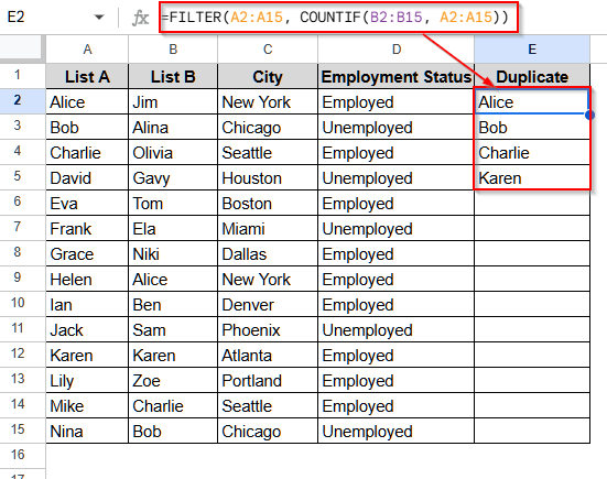
➤ Then, select cell E2 and insert the following formula:
=FILTER(A2:A15, COUNTIF(B2:B15, A2:A15))
➤ Finally, press Enter on your keyboard, and it will return the duplicate values.
➤ Remember to replace the cell reference (A2:A15, B2:B15, etc.) with your own dataset’s cell reference.
Find Duplicates in Two Columns in Google Sheets with Conditional Formatting
In Google Sheets, conditional formatting can help us find duplicate values in two columns by matching them automatically with the help of the COUNTIF function.
To explain the method, we will use the dataset below.
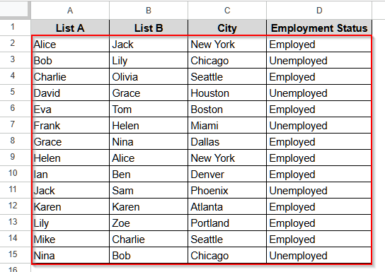
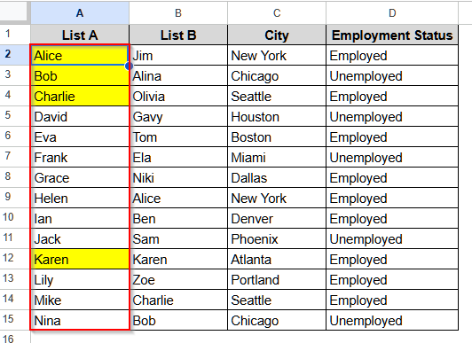
In this dataset, we can see some residents’ names in two columns, column A and column B. We will use a conditional formatting rule on these two columns to find the duplicate values.
Steps:
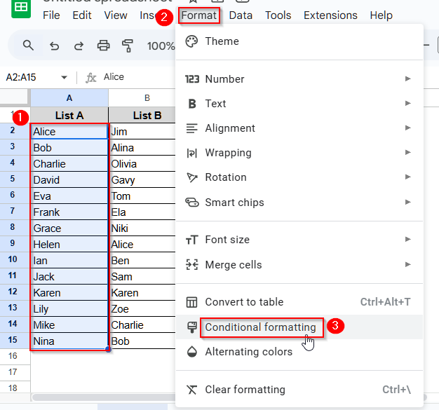
➤ First, select the range A2:A15 by dragging the cursor from cell A2 to cell A15.
➤ Then. Select Format from the top menu. A pop-up will be opened. Select Conditional Formatting from that pop-up.
➤ Now, you will see another window open on the rightmost side of the dataset. In that window, under the Format cells if… option, you will see a drop-down arrow.
➤ Click on the drop-down arrow, and a list of options will open. Scroll to the bottom of that list and select the Custom formula is option.
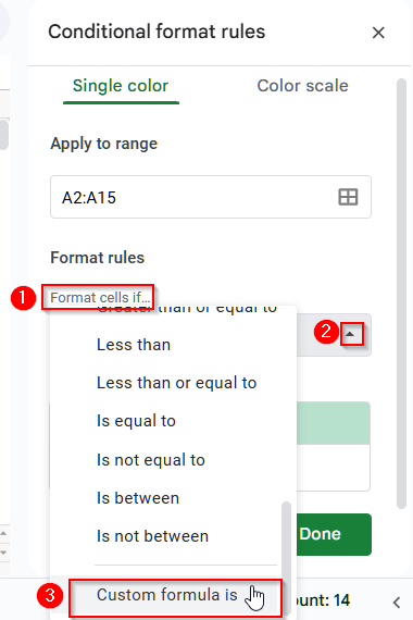
➤ Now, select the Value or formula option.
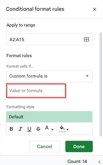
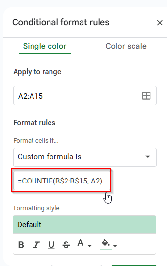
➤ In that box, write down this formula:
=COUNTIF(B$2:B$15, A2)
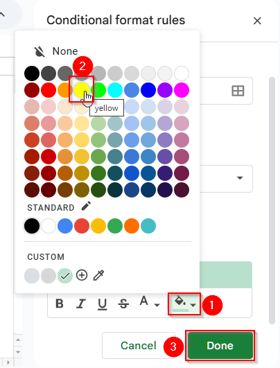
➤ Now, from the Formatting style option, you can customize the style by changing the fill color or making the text bold, etc. To change the color, click on the color square icon on the rightmost side. Pick any color you like and click Done.
➤ Now, you will see all the duplicates values between column A and column B has been highlighted with yellow color in column A.
Show Duplicates in Google Sheets with the COUNTIF Function
Combining the COUNTIF and IF functions, we can find out the duplicates in two columns by counting how many times a value appears in them. It also allows us to customize the return value, like Yes/No, 0/1, etc.
Below, we have explained how you can use the COUNTIF function to find duplicates in two columns in a Google Sheets dataset.
Steps:
➤ First, select cell E1 and write a name like Duplicate for it.
➤ Now, click on cell E2 and insert the following formula:
=IF(COUNTIF(B$2:B$15, A2), “Yes”, “No”)
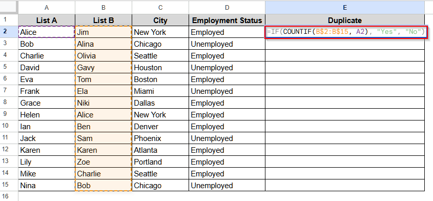
➤ Press Enter and then drag the cursor down to fill all the values.
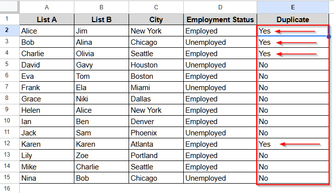
From the result, we can see, the duplicate names in column A in respect to column B, returned Yes.
Using FILTER Function to Find Duplicates in Two Columns
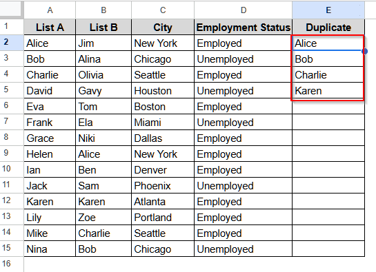
If you want to see only the duplicate values between two columns exclusively, the FILTER function is the best choice. This function not only identifies the duplicate values, but also returns them in a separate column. Thus, it becomes clearer to visualize and easier to find the duplicate values.
Let’s go through the explanation below to know how to use this FILTER function to find duplicate values in Google Sheets.
Steps:
➤ At first, select cell E1 and give it a name.
➤ Then, select cell E2 and insert the formula as below:
=FILTER(A2:A15, COUNTIF(B2:B15, A2:A15))
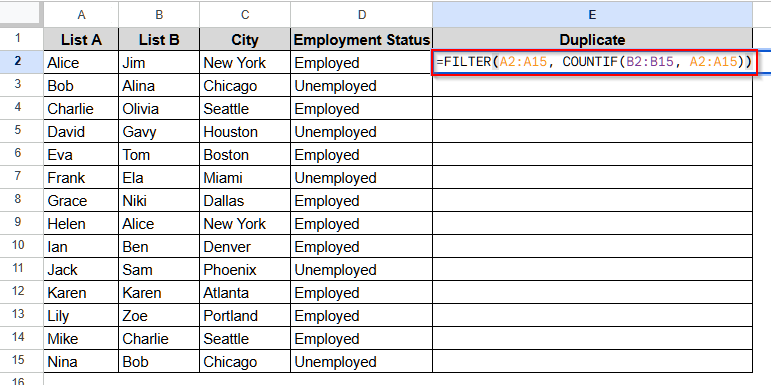
➤ Finally, press Enter, and it will return all the duplicate values.
Frequently Asked Questions
Can I Count the Duplicate Entries Between Two Columns in Google Sheets?
Yes, using the ARRAYFORMULA function, you can easily count the number of duplicate entries between two columns in Google Sheets. Select an empty cell and insert the following formula: =ARRAYFORMULA(SUM(COUNTIF(B2:B, A2:A))). Press Enter, and you will see the total number of duplicate values between the columns.
Can I Find Duplicate Values across Multiple Columns in Google Sheets?
Absolutely. Using the CONDITIONAL FORMATTING function, we can easily find out the duplicate values across multiple columns. Select the range of data you want to find the duplicate values, let’s say, the range is A2 to B15. Look at the top menu of the dataset and select Format > Conditional Formatting > Format cells if … > Custom formula is. Now, inside the Value or formula box, write down the formula: =COUNTIF($A$2:$B$15, A2)>1 and choose any highlight color. You will see that all the duplicate values across this range will be highlighted.
Can I Prevent Duplicate Entries in Real-time in Google Sheets?
Yes, with the help of the Data Validation function, you can easily prevent duplicate entries in real-time. Select the data range you want to apply Data validation to, let’s say, it is A1:A100. Now, from the top menu of the dataset, select Data> Data validation. A new window will open up. Click on Add rule and under Criteria, select the Custom formula is option. Then, in the Formula box, insert this formula: =COUNTIF($A$2:$A$100, A2)=1. Then, click Save. Now, this will prevent you from entering duplicate values in that range.
Wrapping Up
In this article, we have learned to use CONDITIONAL FORMATTING, COUNTIF, and FILTER functions to find duplicates in two columns in a Google Sheets dataset. Try these methods and share your experience with us. Also, do not hesitate to reach out in comments if you have any queries.

