When you are working in Google Sheets, you will often need to calculate or show percentages. Specially when you are summarizing survey responses, applying discounts, tracking sales growth, reviewing students’ grades, or calculating taxes. This article provides the most practical methods to add, format, and visualize percentages in Google Sheets automatically.
Steps to Format Numbers as Percentages:
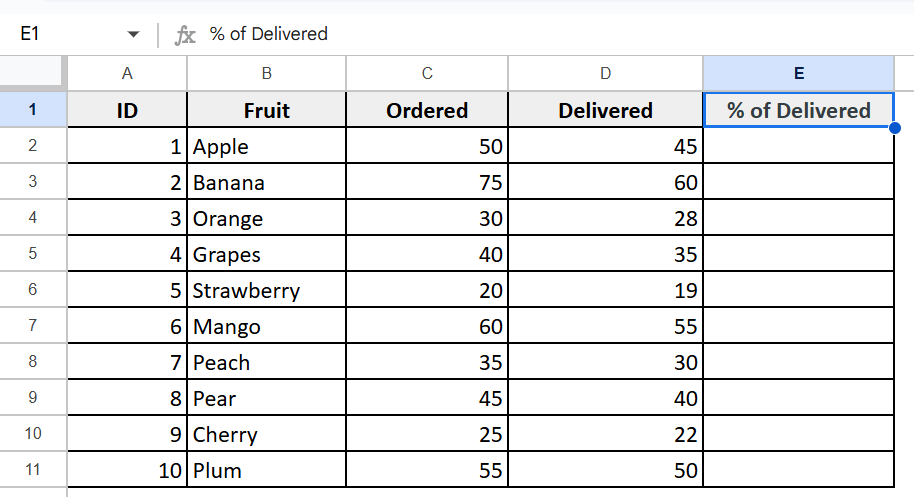
➤ Insert a new column E and name it as % of Delivered
➤ In E2 enter =D2/C2
➤ Format as Percentage from the toolbar.
➤ Drag down the formula.

In this article, we will explore several practical methods to add percentages automatically in Google Sheets. We will use techniques like the basic division formula, inline text-based percentage condition using the IF function and SUM, COUNTIF, and visual indicators through SPARKLINE bars.
Using Basic Percentage Formula
The basic percentage formula in Google Sheets is one of the most commonly used methods for calculating percentages. It works by dividing one value by another and then multiplying the result by 100 to get the percentage.
In the following dataset, we’ll find out the percentage of the delivered fruits based on the ordered ones.
Steps:
➤ Insert a new column E and name it as % of Delivered
➤ In cell E2 enter the following formula:
=D2/C2

➤ Format as Percentage from the toolbar.

➤ Drag down the formula, and it will return percentage values sequentially.

Calculate Percentage with SUM and Division Formula
This method works by summing all delivered units and dividing them by the total ordered units, giving a single percentage that reflects overall fulfillment. It is very useful for summary reports, dashboards, or when you want to quickly assess total progress without reviewing individual entries.
Steps:
➤ Insert a new column E and name it as % of Delivered.
➤ In cell E2, enter the following formula:
=SUM(D2:D11) / SUM(C2:C11)

➤ Drag down the formula, and it will return percentage values sequentially.

To Calculate the Percentage of Total
This method is used to determine what portion each individual value contributes to the total sum of a dataset. We’ll add two more extra columns E & F here and then calculate the percentage of the total orders & also the percentage of the total deliveries.
Steps:
➤ In cells C12 and D12, find out the following results first:
Total Ordered:=SUM(C2:C11) and Total Delivered: =SUM(D2:D11)

➤ Add new columns and name them % of Total Ordered in column E and % of Total Delivered in column F.

➤ Select columns E and F, then Format as Percentage from the toolbar.

➤ Enter the percentage formulas in E2 (for % of Ordered): =C2 / $C$12 and In F2 (for % of Delivered): <strong>=D2 / $D$12</strong>
➤ Drag down the formulas to rows 3–11.

Calculate Percentage Based on Criteria
In Google Sheets, percentage calculations based on criteria are useful for analyzing how much of a dataset meets a specific condition, like what percentage of students passed or how many orders came from a certain region. We can do this by combining the IF function with a percentage calculation.
Steps:
➤ Insert a new column E and name it as % of Delivered
➤ In E2, enter =D2/C2 and drag down to E11 and format as a percentage.

➤ To calculate the percentage of fruits delivered greater than or equal to 90%:, enter the following formula in cell F2, go to Format > Number > Percent
=COUNTIF(E2:E11, “>=90%”) / COUNTA(E2:E11)

➤ It will return the percentage of entries.
Create a Percentage Bar Using SPARKLINE
The SPARKLINE function in Google Sheets inserts tiny, in-cell charts that summarize data visually. By using the bar chart type and setting the maximum value to 1 or 100%, you can create a horizontal progress bar that fills proportionally to the percentage value you want to represent. This visual signal makes it easy to spot trends and performance without scanning numbers.
Steps:
➤ In a new column, E2 enter the formula
=SPARKLINE(D2/C2, {“charttype”,”bar”; “max”,1})

➤ Drag down for all rows. It will return a horizontal bar in the rest of the cells.

Show Conditional Output Based on Percentage in a Text Formula
This method uses the IF function to compare the delivered value against the ordered value. If the two values are equal, meaning 100% of the order has been delivered, the formula shows Done. Otherwise, it shows Pending. This is an effective method to communicate status when numeric percentages are not necessary.
Steps:
➤ Insert a new column E and name it as Delivery Status.
➤ In E2 enter this formula
=IF(D2/C2=1, ” Done”, ” Pending”)

➤ Press Enter and drag the fill handle down to apply the formula to the entire column.

Frequently Asked Questions
How do I calculate a percentage of two numbers in Google Sheets?
Use the formula =part/total and format the cell as a percentage from the toolbar.
How do I display percentages with decimal places?
After calculating the percentage, use the Increase Decimal button in the toolbar to show more decimal places.
How do I calculate the overall percentage for multiple rows?
Use =SUM(delivered_range)/SUM(ordered_range)
Wrapping Up
Calculating percentages in Google Sheets makes data analysis clearer and more effective. This article covered simple formulas status indicators and overall calculations and visual tools to help you work smarter.Using these methods will save time, reduce errors and enhance your reports effortlessly.