
When you want to maintain clean data in Google Sheets, you may need to trim unwanted characters from the end of text strings. Removing the last character, like extra punctuation, stray letters, spaces, or numbers, helps to keep your data organized and tidy.
It is not a very difficult task, as Google Sheets offers multiple simple formulas. In this guide, we’ll show you how you can remove the last character from one cell or multiple cells using two functions: the LEFT and the ARRAY formula.
➤ Google Sheets has simple formulas to remove the last character automatically from one or more cells.
➤ The LEFT function: It removes the last character by trimming based on the specified number of characters.
➤ The ARRAY formula: It removes the last character from a range of cells and removes the last one from each cell.
Removing the Last Character from Google Sheets using the LEFT Function
The LEFT Function in Google Sheets is a simple but powerful method when you need to remove the last character from a string. It allows you to delete the substring from the left side of your data based on a specified number of characters.
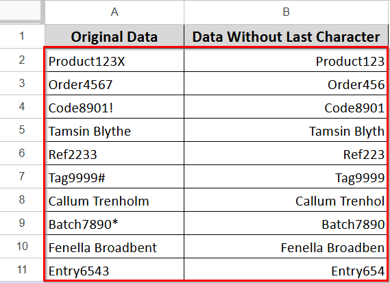
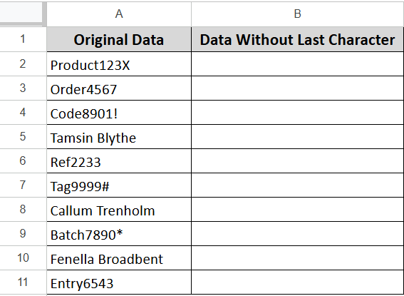
In the following dataset, we have a mix of random text values containing a mix of letters, numbers, and symbols. We are going to remove the last character using the LEFT Function from each entry.
Steps are below:
➤ Insert the following formula in the B2 cell.
=LEFT(A2, LEN (A2)-1)
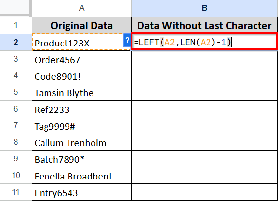
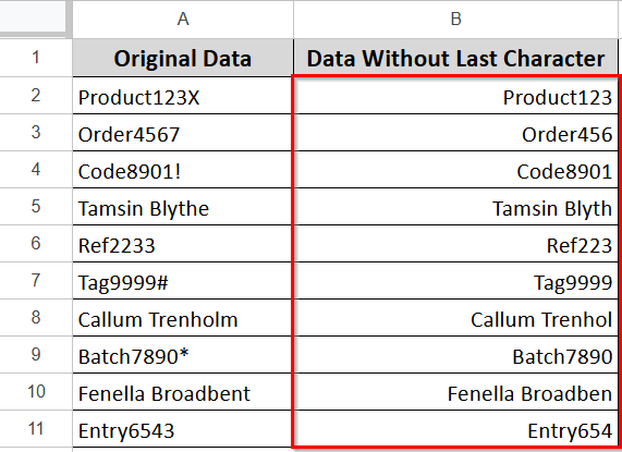
➤ Press Enter, and the formula will remove the last character from the string in cell A2.
➤ Google Sheets suggests an Autofill pop-up. Check it or just press Ctrl + Enter to fill the rest.
Here is the short breakdown of the formula:
➥ The LEFT function takes text from the start of a cell.
➥ LEN counts how many characters are in the cell.
➥ LEN(A2) - 1 means you're telling it to take the last character.
Removing the Last Character From Google Sheets Using the ARRAYFORMULA Function
If you are working with a large dataset, an ARRAYFORMULA function lets you remove the last character from a range of cells. This way, you don’t have to apply the formula individually to each cell.
Follow the steps below to do so:
➤ Enter the formula below in the B2 cell.
=ARRAYFORMULA(LEFT(A2:A11, LEN(A2:A11) – 1))
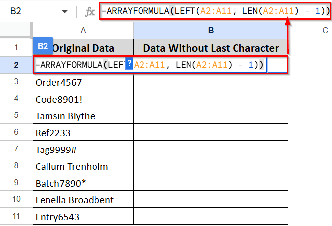
➤ Press Enter. You will see the results all at once.

Here is a short explanation of the formula.
➥ LEFT takes text from the start of a cell.
➥ LEN counts how many characters are in each cell.
➥ A2:A11 is the entire range of the cells.
➥ LEN(A2:A11) - 1 means it counts all the letters in each cell, then subtracts one to remove the last letter.
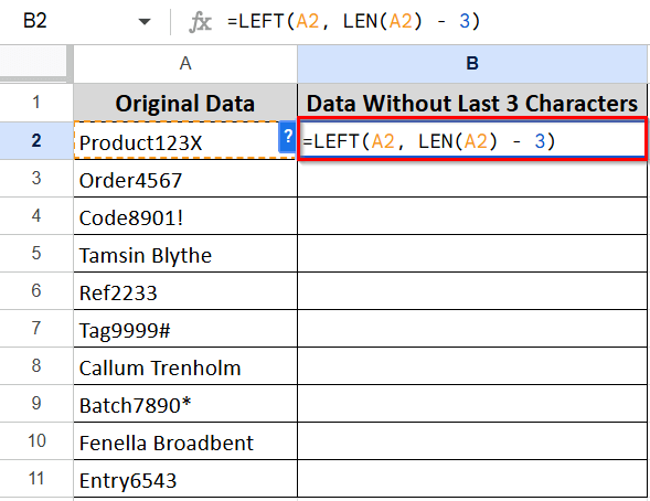
Removing the Last ‘n’ Character From Google Sheets
You can also use the LEFT function with the LEN function to remove the last ‘n’ characters from Google Sheets. The formula is: =LEFT(cell, LEN(cell) – n). Here ‘n’ is the number of characters you want to remove from the text.
Steps are below.
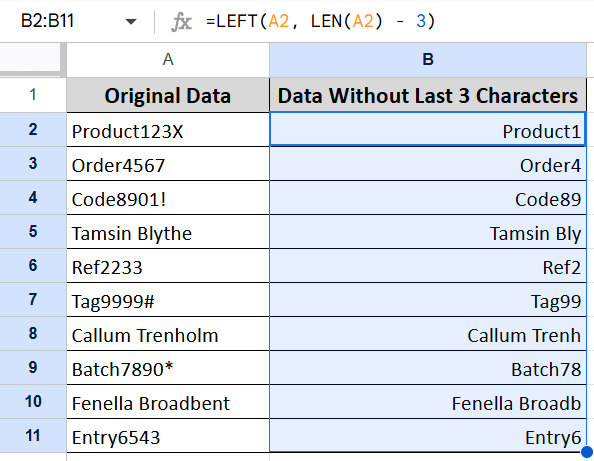
➤ Enter the below formula in the B2 cell to remove the last 3 characters from the text in cell A2.
=LEFT(A2, LEN(A2) – 3).
➤ Press Enter. The formula will return the text in cell A2 with the last 3 characters removed. Use the Autofill option to apply the formula to the rest of the cells.
Frequently Asked Questions
How do I remove the last name in Google Sheets?
You can remove the last name in Google Sheets using the formula below:
=INDEX(SPLIT(A1, ” “), 1). For example, if the A1 cell has “John Smith”, the formula returns “John”. This formula gets only the first name and works for two-part names.
How do I remove the last edit in Google Sheets?
You can remove the last edit in Google Sheets following the steps below:
➤ Click the Undo button. It appears as a backward arrow on the toolbar at the top. Or
➤ Press Ctrl + Z for Windows and Cmd + Z for Mac. It will undo the last changes.
How do I remove letters in Google Sheets?
You can remove letters in Google Sheets using the REGEXREPLACE formula.
➤ Enter the =REGEXREPLACE(A1, “[A-Za-z]”, “”) in A1 cell.
➤ The formula will remove all the alphabetic characters from the cell. For instance, if the A1 cell contains “A123B”, the formula will return “123”.
How do I remove special characters in Google Sheets?
You can remove the special characters in Google Sheets with the formula below, based on your needs.
- =REGEXREPLACE(A1,”[^A-Za-z]+”,””: To remove everything except letters.
- =REGEXREPLACE(A1, “[^0-9a-zA-Z]”, “”): To remove everything except numbers and letters.
- =REGEXREPLACE(A1, “[!$%]”, “”): To remove specific special characters.
How do you remove the last comma in Google Sheets?
Follow the steps below to remove a comma in Google Sheets:
➤ Select the cell where you want the result to appear.
➤ Enter the formula: =SUBSTITUTE(A1, “,”, “”)
➤ Press Enter. It will remove all commas from the text in A1.
Wrapping Up
In this quick tutorial, we have covered three easy ways to remove the last character in Google Sheets using formulas. You can apply these techniques to clean and manage your data efficiently. Download the sample sheet to practice, and let us know how it enhances your productivity.