
When you import large sets of data from surveys, CRMs, or databases into Google Sheets, having duplicate data could screw up calculations, give you wrong overviews, or just make the sheet look cluttered. Usually people want a dynamic, real-time solution instead of a one-time removal, they often look for a formula that will help them get rid of duplicates. Formulas that remove duplicates ensure that your data updates automatically every time you add a new value.
To remove duplicates in Google Sheets using UNIQUE function, follow these steps:
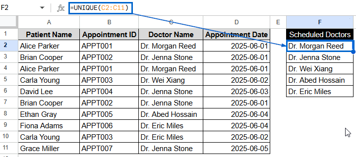
➤ Select a blank column. In this case, F2.
➤ Enter the formula:
=UNIQUE(C2:C11)
➤ Press Enter to get a unique list of doctor names
In this piece, we’ll take a look at different ways to use formulas to get rid of duplicates in Google Sheets. We’ll talk about the built-in UNIQUE function, how to use FILTER to make more complex combinations, how to deal with duplicates across multiple columns, and how to use conditions to get more controlled outputs for advanced users.
Using UNIQUE Function to Remove Duplicates
Google Sheets has a built-in function called UNIQUE that helps you get rid of duplicate entries in a list or dataset. This can be the easiest way to get rid of those full-row duplicates while keeping the first one. This method is helpful if you only want to get back one copy of each unique appointment.
In the following dataset, there is a list of clinical appointments, and some names show up more than once. We will use the UNIQUE formula to remove these duplicates. This formula only shows the first instance of each name and overlooks the rest.
Steps:
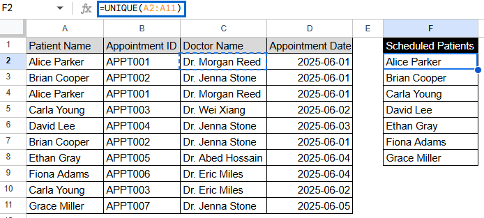
➤ Select a blank cell named F2.
➤ Enter the formula:
=UNIQUE(A2:A11)
➤ Press Enter to get a unique list of patient names.
Note:
UNIQUE is case-sensitive. It sees Dr. Morgan Reed and dr. morgan reed as two separate entries.
Applying UNIQUE with FILTER to Remove Duplicates Based on Criteria
If you only want to remove duplicates from a particular portion of your data that meets certain criteria, this method works well. It doesn’t look at the whole dataset; instead, it filters the rows initially based on things like category, status, or value. Then it uses the UNIQUE function to get only the unique results from that filtered group.
Steps:
➤ Select an output column, e.g., F.
➤ Use the formula:
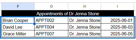
=UNIQUE(FILTER(A2:D11, C2:C11=”Dr. Jenna Stone”))
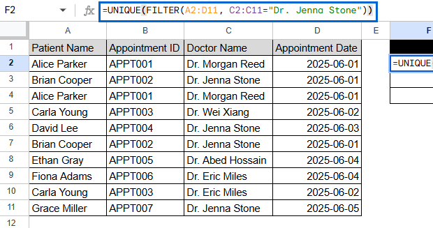
➤ Press Enter to see a filtered list of unique items.
Note:
Before removing duplicates, FILTER lets you set conditions like numerical ranges, text matches, and so on. This method works very well for dashboards and conditional reports.
Operating UNIQUE Across Multiple Columns to Remove Entire Duplicate Rows
You might want to make sure that an entire row is unique, not just the values in it. Ideally, you can use the UNIQUE function to check whole rows by entering more than one column.
Steps:
➤ Select a blank cell where you want the clean result. Here, cell F2.
➤ Enter the formula:
=UNIQUE(A2:D11)
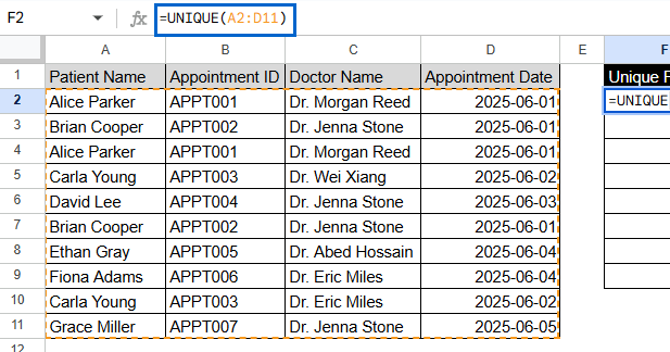
➤ Hit Enter. It will show unique patient appointments with doctors.
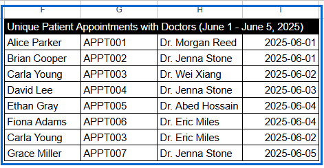
Note:
Each row is treated as a whole, so rows that have the same values in all columns will be deleted. It doesn’t work for duplicates that are only part of the original.
Remove Duplicates by using QUERY Function
The QUERY function lets you get rid of duplicate entries and gives you greater flexibility over how you filter, sort, and choose columns. This method comes in handy if you want to filter in SQL style or use logic, like sorting or skipping headers.
Aggregation (AGG) like MIN is used with GROUP BY to combine rows that have the same values in grouped columns by summarizing other columns.
Steps:
➤ Select a new column or cell. Here F2.
➤ Enter this formula:
=QUERY(A2:D11, “SELECT A, B, C, MIN(D) GROUP BY A, B, C LABEL A ”, B ”, C ”, MIN(D) ””, 0)
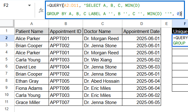
➤ Press Enter to view the cleaned list.
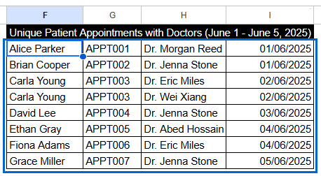
Note:
You need aggregation (AGG) because QUERY can’t group rows without at least one column being summarized.
Display Only First Instances Using ARRAYFORMULA and MATCH Functions
This method is for more experienced users who want to highlight or take out just the first instance of each duplicate while keeping the whole row of data. This is ideal if you want to keep the original formatting or order of the rows.
Steps:
➤ Click a blank column, F2
➤ Type this formula:
=ARRAYFORMULA(IF(MATCH(A2:A11&B2:B11&C2:C11&D2:D11, A2:A11&B2:B11&C2:C11&D2:D11, 0)=ROW(A2:A11)-ROW(A2)+1, A2:A11, “”))
➤ Press Enter. Patients scheduled in June will be shown in column F.
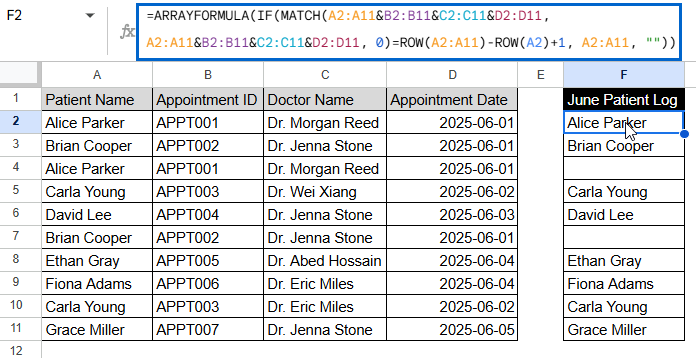
Note:
This approach doesn’t collapse the list; it keeps the structure and only shows the first hits. It’s superb when keeping the order of the rows is important.
Frequently Asked Questions
What is the best formula to remove duplicates in Google Sheets?
The UNIQUE function is the most effective method to remove duplicates instantly. It automatically removes duplicate entries from your data range.
Does the UNIQUE function update automatically?
Yes, the UNIQUE function automatically updates when the data source changes. It “spills” results into adjacent cells, which are updated to reflect changes in the original data.
What do I do if the UNIQUE function gives me a blank cell?
If your formula returns a blank result, it usually means that it is pointing to empty cells or that the range has no data. Check that the input range is correct and that it has real duplicate values to filter.
Does UNIQUE consider text cases when removing duplicates?
Yes, the UNIQUE function is case-sensitive. “Data” and “data” will be considered two different things.
Can I sort the unique results?
Yes. To show the unique values in order, you can put the formula inside a SORT function like this:
=SORT(UNIQUE(A2:A11)).
Concluding Words
Using the UNIQUE function and its variations in Google Sheets makes it easy and powerful to get rid of duplicates. These formula-based methods are a flexible, hands-free way to keep your sheets clean and accurate, whether you’re cleaning up raw survey data or making reports. You can change how you remove duplicates to fit any workflow or data condition by using functions like FILTER, QUERY, and ARRAYFORMULA together.