Rounding in Google Sheets means adjusting a number to make it simpler. Instead of showing exact values like 136 or 278, you can round them to a cleaner number such as 200 or 300. Usually, we need to round numbers when working on budgets, price lists, sales targets, inventory estimates, or financial summaries where you want to avoid small variations.
Rounding up to the nearest 100 is often used in financial planning and bulk pricing. It helps keep data easy to scan, avoids underestimation, and improves consistency across your spreadsheet.
In this article, we’ll learn how to round up numbers to the nearest 100 in Google Sheets using multiple methods.
The CEILING function is the simplest way to round numbers up to the nearest 100 in Google Sheets.
Here’s a simple guide to apply this method:
➤ Open your dataset in Google Sheets.
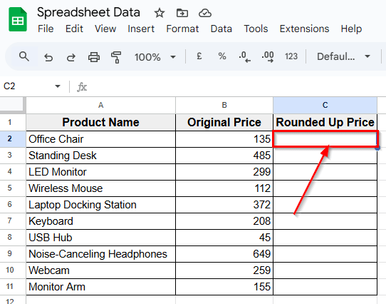
➤ Click on cell C2, where you want the first rounded value to appear.
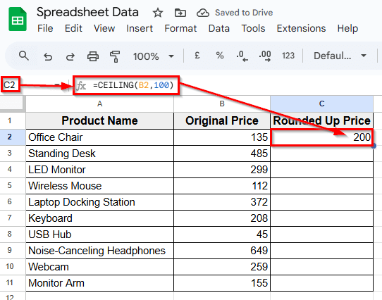
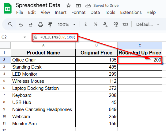
➤ Type this formula =CEILING(B2, 100)
➤ Press Enter. The result will be 200, since 135 rounded up to the nearest 100 is 200.
Using the CEILING Function To Round Up Nearest 100
In the following dataset, we use a product list that shows the original prices of various office items. There are three columns labeled Product Name, Original Price, and Rounded Up Price. Column A includes the product names, Column B shows their original prices, and Column C is currently empty.
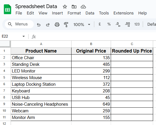
We’ll use this third column to round up each original price to the nearest 100 using different formulas in Google Sheets.
The CEILING function is the simplest way to round numbers up to the nearest 100 in Google Sheets. It increases a number to the next closest multiple of a value you choose.
In this case, we’ll round each price in Column B up to the next 100 using this function.
Here’s a simple guide to apply this method:
➤ Open your dataset in Google Sheets.
➤ Click on cell C2, where you want the first rounded value to appear.
➤ Type this formula
=CEILING(B2, 100)
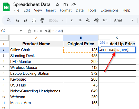
➤ Press Enter. The result will be 200.
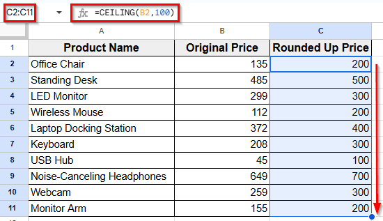
➤ Now click on the bottom-right corner of the cell and drag it down through the rest of Column C.
➤ This will apply the same formula to the rest of the product prices, rounding each one up to the next multiple of 100.
Applying ROUNDUP Function With Math Logic
You can also use the ROUNDUP function combined with simple math logic to round numbers up to the nearest 100. It works by dividing the number, rounding it up, and then multiplying back to get the desired result.
Here’s how to do it step-by-step:
➤ Open your dataset in Google Sheets.
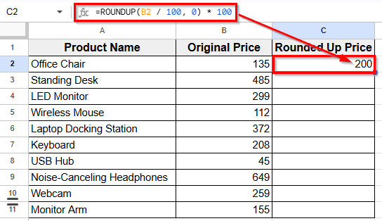
➤ Click on cell C2, where you want the first rounded value to appear.
➤ Type this formula
=ROUNDUP(B2 / 100, 0) * 100

➤Next, press Enter. The result will be 200.
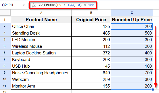
➤ Finally, drag the fill handle down to fill the formula across the other rows in Column C.
➤ This copies the formula to the other rows, rounding each number up to the nearest 100 using the same logic.
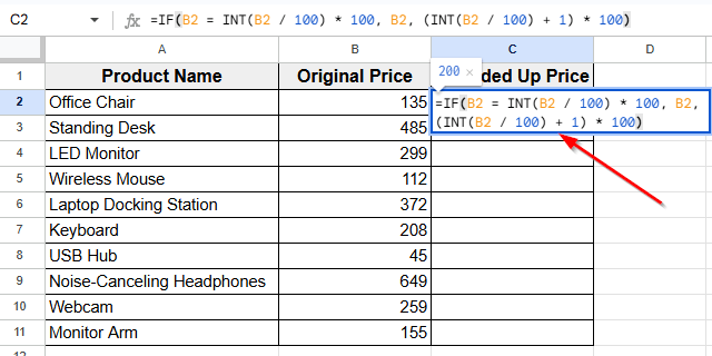
Using IF and INT for Custom Rounding
If you prefer a manual way to round numbers up to the nearest 100 using basic functions, combining IF and INT works well. This method checks if the number is already a multiple of 100 and rounds up only if needed.
In this method, we’ll apply this formula to the numbers in Column B and show the rounded results in Column C.
Here’s a simple step-by-step guide to do it:
➤ Open your dataset in Google Sheets.
➤ Click on cell C2, where you want the first rounded value to appear.
➤ Type this formula
=IF(B2 = INT(B2 / 100) * 100, B2, (INT(B2 / 100) + 1) * 100)
➤ Press Enter.
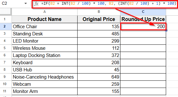
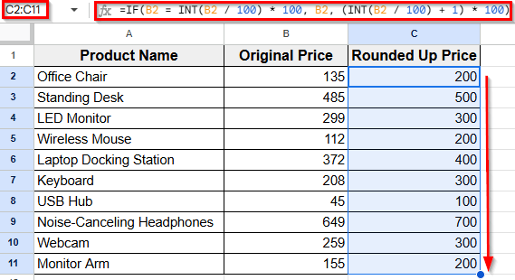
➤ Drag the fill handle at the bottom-right corner of C2 down through the rest of Column C.
➤ This copies the formula to other rows, rounding each number up to the nearest 100 manually by checking each case.
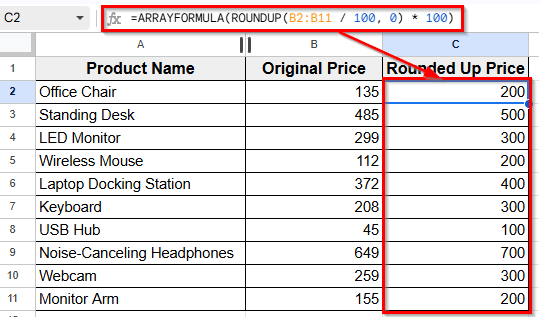
Combine ARRAYFORMULA and ROUNDUP Function for Auto-Fill Rounding
If you want to round numbers up for an entire column automatically, combining the ARRAYFORMULA function with ROUNDUP is a great way to do it. This lets you apply the formula once and fill the whole column without dragging.
Here’s how to use this method:
➤ Open your dataset in Google Sheets.
➤ Click on cell C2, where you want the rounded results to begin.
➤ Type this formula
=ARRAYFORMULA(ROUNDUP(B2:B11 / 100, 0) * 100)
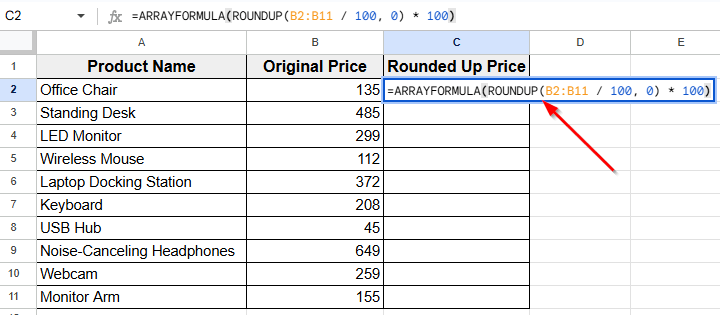
➤ Press Enter. This formula rounds up each value in Column B to the nearest 100 and automatically fills Column C with the results.
Frequently Asked Questions
What is the formula for roundup?
To round a number up in Google Sheets, the most common formula is the ROUNDUP function. It increases a number to the next specified place value.
Here’s how to use it:
➤ Open your Google Sheet.
➤ Click on the cell where you want the rounded number to appear.
➤ Type the formula like this =ROUNDUP(B2, 0)
➤ Press Enter. This will round up the value in cell B2 to the next whole number.
How do I round up to 100 in Google Sheets?
To round up to the nearest 100, you can use the CEILING function.
Here’s how to do it:
➤ Open your Google Sheet.
➤ Click on the cell where you want the result.
➤ Type the formula =CEILING(B2, 100)
➤ Press Enter. This will round up the number in cell B2 to the next multiple of 100.
Wrapping Up
When you’re working with large numbers in Google Sheets, rounding the numbers can make your data much easier to read and work with. Using the right rounding method saves time and keeps things consistent while organizing sales figures, budgeting, or preparing reports.
The formulas we’ve mentioned earlier are simple and effective at the same time. You can choose the method that fits your workflow best. For a quick solution use the CEILING function, or try ROUNDUP with a bit of math for more control.
Also, you can apply the ARRAYFORMULA function combined with ROUNDUP to get automatic results. And for those who like manual logic, combining IF and INT works just as well.

