
When you use Google Sheets, you often encounter datasets with several values in one cell, like names, product codes, or categories, separated by commas, spaces, or hyphens. If you only want the first part of that split value, like the first name from a full name or the first item in a list, then this article should answer all your queries. People often use this method to clean up data, organize CRM data, or prepare customer groups for marketing campaigns.
To split a cell and return only the first value:
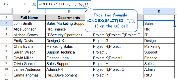
➤ Select the output cell (e.g., D2).
➤ Type the formula:
=INDEX(SPLIT(B2, “,”), 1) on the D2 cell
➤ Press Enter to see the first part of the text in cell B2, with commas separating it. To get the second or third part, change the number to 2 or 3.
➤ Use the Fill Handle to apply the formula down the column.
We’ll look at different ways to split a cell and get just the first item in Google Sheets in this article. We’ll also talk about how to use the SPLIT function, combine SPLIT and INDEX functions, then again use another combination of LEFT and SEARCH functions, and dynamic methods like the ARRAYFORMULA function to handle different delimiters or more than one value.
Use the SPLIT Function Only
The SPLIT function in Google Sheets splits text in one cell into two or more cells based on a certain character or group of characters called the delimiter. It helps a lot to put names, tags, categories, and other grouped data into separate columns.
SPLIT Function Syntax:
=SPLIT(text, delimiter, [split_by_each], [remove_empty_text])
Steps:
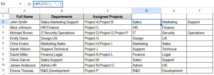
➤ Select the output cell where you want the split values to appear (e.g., D2, E2, and F2).
➤ Type the formula:
=SPLIT(B2, “,”)
➤ Press Enter. The data will be organized into three columns; D, E, and F. The first items of the column are arranged in the D column.
Note:
Make sure there are always enough empty cells to the right of the formula so that the split results don’t overwrite any existing data. If your delimiter is in the values themselves (not just between them), splitting may not work right.
Using SPLIT and INDEX to Get the First Value
It’s common to keep full names or more than one value in a single cell in real-life datasets. You can use the SPLIT function to break the text into parts and the INDEX function to get the first item.
Formula syntax with SPLIT and INDEX functions:
=INDEX(SPLIT(cell_reference, “delimiter”), 1)
Steps:
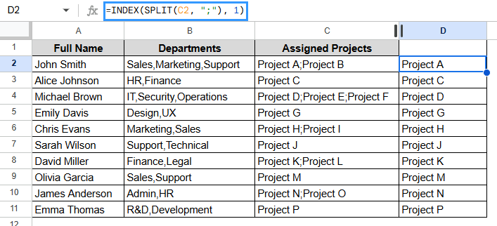
➤ Select the cell for the output (e.g., D2).
➤ Enter the formula:
=INDEX(SPLIT(C2, “;”), 1)
➤ Press Enter to display the first part of the text from cell B2, split by ‘;’. You can change the number (e.g., to 2 or 3) to extract the second or third part instead.
➤ Use the Fill Handle to apply the formula down the column.
Note:
Always make sure the delimiter is the same. You can’t use a comma and a semicolon in the same way. To avoid empty outputs or mistakes, make sure that data is always in the same format.
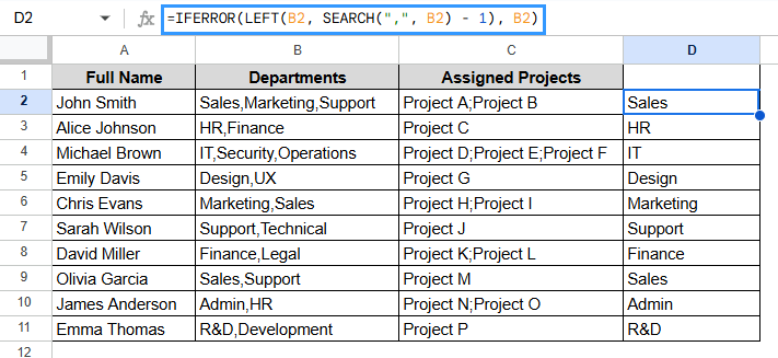
Combining LEFT and SEARCH Functions for Fixed Patterns
If your dataset follows a consistent format, such as first and last names separated by a space, you can use LEFT and SEARCH instead of SPLIT to speed up the process.
LEFT(text, number) gives you a certain number of characters from the beginning of a text string. SEARCH(character, text) helps to find the place in the text where a character, like a dash or space, is.
Steps:
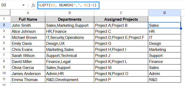
➤ Select the output cell (e.g., D2).
➤ Enter the formula:
=LEFT(B2, SEARCH(“,”, B2)-1)
➤ Press Enter to extract the first item.
➤ Drag down the Fill Handle to apply the formula for all entries.
Note:
This method only works if the original cell has “at least one space” or “,” in it. The formula will give an error if it doesn’t find a space or comma. To avoid this, use `IFERROR()` like this:
=IFERROR(LEFT(B2, SEARCH(“,”, B2) – 1), B2)
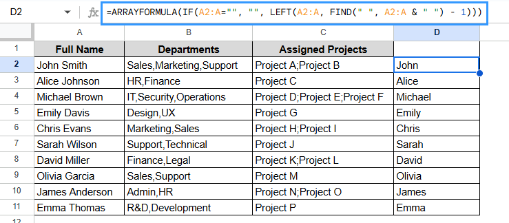
Inserting ARRAYFORMULA for Multiple Cells
You can use ARRAYFORMULA to apply a formula like SPLIT + INDEX to a whole column without having to copy it down by hand. You can also use ARRAYFORMULA and LEFT + FIND to apply a function to a whole range of cells at once. It makes your spreadsheet more useful and scalable by getting rid of repetitive manual work.
Steps:
➤ Select the output cell (e.g., D2).
➤ Type the formula:
=ARRAYFORMULA(IF(A2:A=””, “”, LEFT(A2:A, FIND(” “, A2:A & ” “) – 1)))
➤ Press Enter. It will automatically populate all the rows in Column D where Column B has data.
Note:
This is great for datasets that change a lot and grow a lot. Don’t put this formula next to filled columns because ARRAYFORMULA will fill in all the rows that match.
Frequently Asked Questions
Can I extract only the first item from a list in a cell?
To get the first item, use the SPLIT function with INDEX:
=INDEX(SPLIT(cell, “,”), 1
How can I use different delimiters in the SPLIT function?
You can use any character as a delimiter, like ” “, “,”, “;”, or “/”, depending on how the values are separated.
What if there’s no delimiter in the cell?
You will get an error. To stop this from happening, put the formula in IFERROR():
=IFERROR(INDEX(SPLIT(A2, “,”), 1), A2
How can I auto-apply the split formula for an entire column?
You can use SPLIT and INDEX with ARRAYFORMULA:
=ARRAYFORMULA(IF(A2:A=””, “”, INDEX(SPLIT(A2:A, “,”), 1, 1)))
Does this work on imported or copied data?
Yes, but make sure the delimiters are all the same. You may need to fix the spacing or separators that aren’t standard before you can use the formulas.
Concluding Words
Getting only the first part of a text entry, like a first name or keyword, can make it much easier to work with your data. You can get exactly what you need with SPLIT and INDEX without having to do anything extra. This easy combination saves time and keeps your spreadsheets neat and on topic. It makes your work easier to understand when you’re making contact lists or breaking down product codes.