Working with time data in Google Sheets is essential for tasks like tracking hours worked, logging durations, or calculating total time. This article covers everything from basic formatting to advanced time summing using arrays and auto-updating time logs.
Steps to add time using simple time values:
➤ Select column D (D2:D11).
➤ Go to Format > Number > Duration.
➤ In cell D12 enter =SUM(D2:D11)
➤ Select the total cell D12.
➤ Go to Format > Number > Custom number format and type [h]: mm

In this article, we will explore easy ways to add (sum) time in Google Sheets. You will learn how to add simple time value, use FILTER for flexible summing, sum durations by date with UNIQUE and SUMIF, and sum specific tasks using ARRAYFORMULA with FILTER. These methods will help you quickly calculate total time for projects, tasks, or schedules.
Adding Up Simple Time Values
You can add a simple time value in Google Sheets using the SUM function. These values must be in hh:mm format. To show totals correctly, specially if over 24 hours, you need to format the result cell as hh:mm. This method is ideal for timesheets, study logs, and daily schedules.
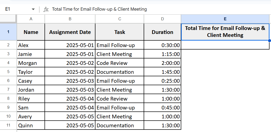
We are using a dataset of students’ tasks with their durations. The first method applied is using the SUM function to calculate the total duration of all tasks.
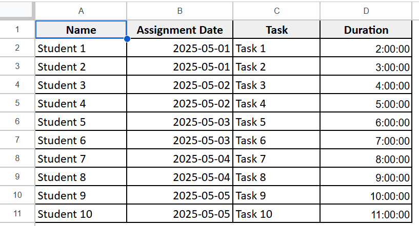
Steps:
➤ Select column D (D2:D11).
➤ Go to Format > Number > Duration.

➤ In cell D12 enter the following formula:
=SUM(D2:D11)
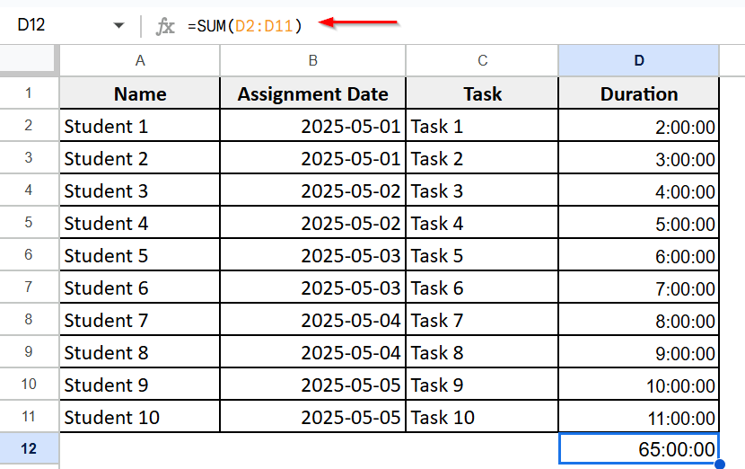
➤ Select the total cell D12.
➤ Go to Format > Number > Custom number format and type [h]: mm
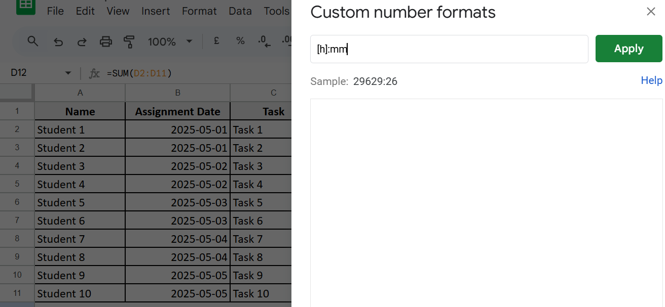
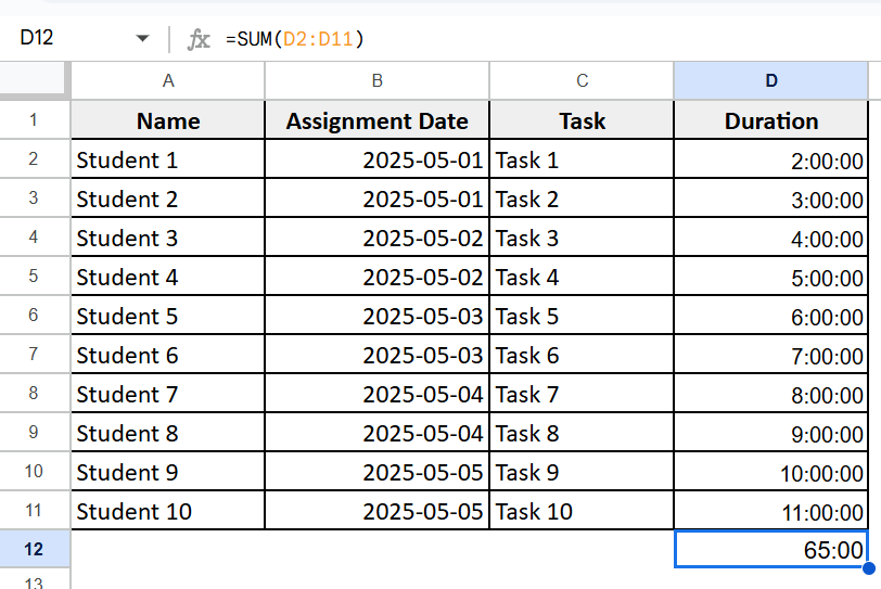
It will return the time in [h]: mm format.
Using FILTER Function for Multiple Conditions
The FILTER function lets you calculate the total time spent on specific tasks or extract data based on several customizable conditions. For example, you can specifically calculate the sum of the “Email follow-up and Client meetings ” by using the FILTER function. This method is useful for dynamically summing durations in task or project management sheets.
Steps:
➤ Select column E and name it as Time for Email Follow-up & Client Meeting.
➤ Select column D (D2:D11).
➤ Go to Format > Number > Duration.
➤ Click on an empty cell, E2 and enter the following formula:
=SUM(FILTER(D2:D11, (C2:C11 = “Client Meeting”) + (C2:C11 = “Email Follow-up”)))
➤ Now sum the duration of tasks that are Client Meeting and Email Follow-up.
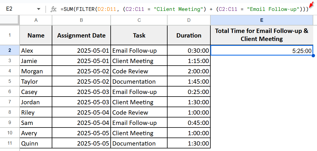
➤ It will return the total time spent on Client Meeting and Email Follow-up.
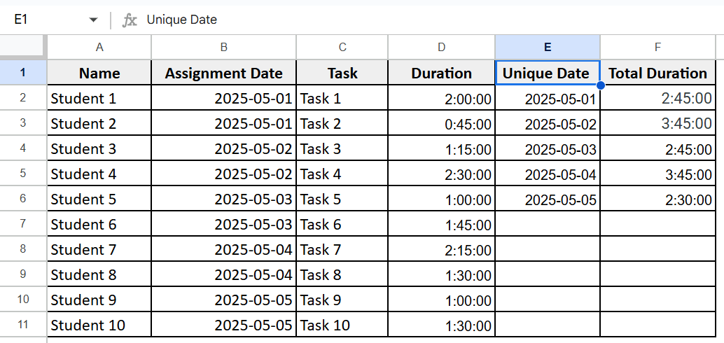
Summing Time Durations by Date Using UNIQUE and SUMIF
When managing task durations or work logs, it’s often useful to calculate the total time spent on each specific date. The combination of the UNIQUE and SUMIF functions in Google Sheets makes this task straightforward and dynamic. The UNIQUE function lists all distinct dates without duplicates, while the SUMIF function adds up duration for each of those dates by matching them in your data.
Steps:
➤ Select column D (D2:D11) and go to Format > Number > Duration.
➤ Click on an empty cell, F2 and enter the following formula:
=UNIQUE(B2:B11)
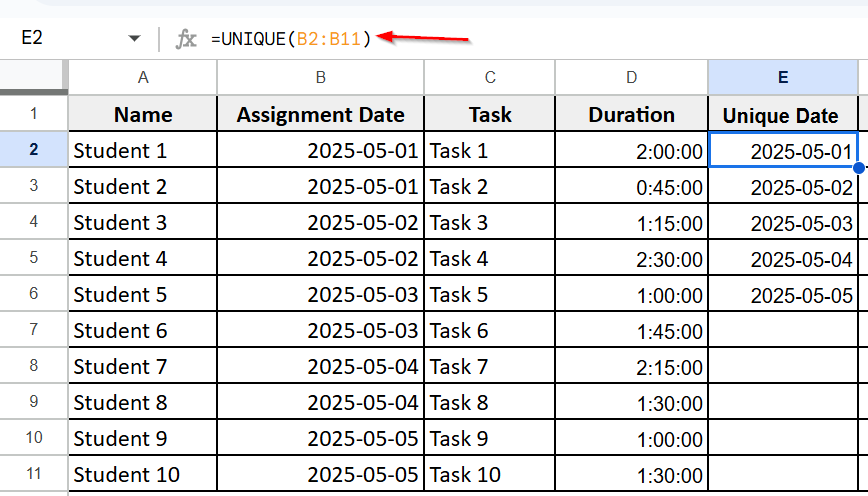
➤ It will return each day only once.
➤ Select G2 and enter the following formula:
=ARRAYFORMULA(IF(F2:F=””, “”, SUMIF(B2:B11, F2:F, D2:D11)))
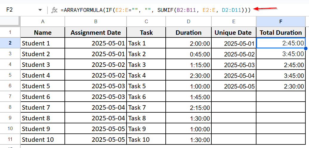
➤ It will return the unique date in column F and the total duration for each date automatically in column G.
Frequently Asked Questions
Can I sum hours and minutes from different sheets?
Yes. Use the formula =Sheet1!A1 + Sheet2!A1 and format the result cell as [h]:mm.
Can I sum time in decimal, like 1.5 hours?
Convert decimal to time using =A1/24 before summing.
What happens if I don’t format the result as Duration?
Google Sheets may display the total as a time of day (e.g., 4:30 AM) instead of a total duration.
Wrapping Up
Summing time in Google Sheets saves effort and reduces mistakes. This article covered simple and advanced methods using formulas and functions to add time values dynamically. These techniques make tracking and calculating total durations for tasks or projects quick and accurate.