
When you use Google Sheets to work with data, you often have to deal with repeated entries, like names, IDs, cities, or any text or numbers that show up more than once. Most of the time, people look for how to count only the unique values so they can get accurate insights without duplicates. This is important for cleaning up data, making summaries, and making smart choices based on unique entries.
To count unique values combining COUNTA & UNIQUE functions in Google Sheets, follow these steps:
➤ Click on a blank cell where you want to display the count. In this case, F2.
➤ Type the formula:
=COUNTA(UNIQUE(A2:A11))
➤ Press Enter to get the count of unique values.
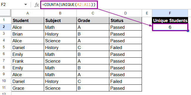
The response is 6 because there are 6 different students on the list, even though some names show up more than once.
In this article, we’ll look at a few different ways to count unique values in Google Sheets. These include basic formulas, case-sensitive methods, condition-based counts, and counting unique values across multiple columns or whole datasets.
Using COUNTA and UNIQUE to Count Unique Values
One of the easiest ways to count unique values in any range is to use COUNTA and UNIQUE together. It gets rid of duplicates and tells you how many unique entries are left.
Let’s say, you have a dataset of students’ grades and pass/fail status in different subjects. Combining COUNTA and UNIQUE helps you find out how many different students, subjects, or student-subject combinations there are without counting the same ones more than once.
Steps:
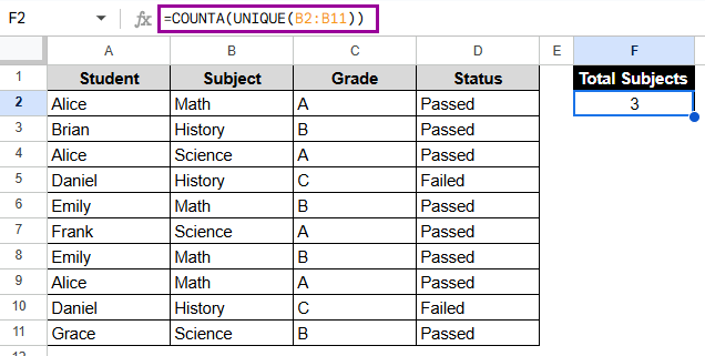
➤ Click on a blank cell, e.g. F2.
➤ Type the formula:
=COUNTA(UNIQUE(B2:B11))
➤ Press Enter.
Note:
It is case-insensitive and skips over empty cells.
Applying COUNTUNIQUE Function to Count Unique Values
COUNTUNIQUE is a built-in function that lets you count the number of unique values in a single step. It’s ideal for quick summaries. Unlike COUNTA(UNIQUE), which returns the same result in two steps, COUNTUNIQUE handles everything in one function.
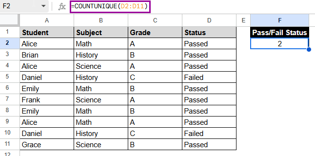
This method counts how many different status values (Passed and Failed) are in the Status column.
Steps:
➤ Select a blank cell. Here, F2.
➤ Enter the formula:
=COUNTUNIQUE(D2:D11)
➤ Press Enter to view the result.
Note:
It counts both letters and numbers. It is case-insensitive, though, like COUNTA, and it ignores blanks.
Filtering Unique Values with Multiple Criteria
The FILTER function lets you sort data by more than one condition. With this method, you have full control over the results because you cut down the details before looking for identity. It helps with school data, analyzing performance, and filtered reports.
In this method, we’ll extract the number of students who uniquely meet both conditions: having an A grade and a Passed status.
Steps:
➤ Select the blank cell, F2.
➤ Enter the formula:
=COUNTA(UNIQUE(FILTER(A2:A11, C2:C11=”A”, D2:D11=”Passed”)))
➤ Press Enter.
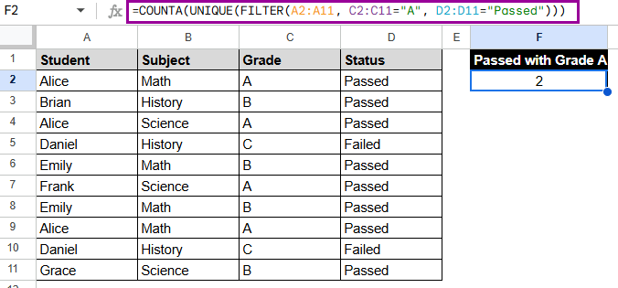
Only 2 people, Alice and Frank, passed their contemporary subjects with Grade A.
Note:
To count a row, all of these conditions must be true. You can always change the filters to fit your dataset.
Count Unique Values Using COUNTIF and SUMPRODUCT
You can also use the COUNTIF and SUMPRODUCT functions together to count unique values in Google Sheets. This method works well by giving each repeated entry a fractional value and then adding them all up to get the total number of unique values.
Suppose your dataset is about electronics stores, where the columns show the Date, Customer Names, and Store Items. Here, we want to know how many different kinds of products were sold in Store 1.
Steps:
➤ Click on a blank cell. In this case, F2.
➤ Enter the formula:
=SUMPRODUCT(1/COUNTIF(C2:C11, C2:C11))
➤ Press Enter. The answer will be 6, which is the number of unique things in Store 1.
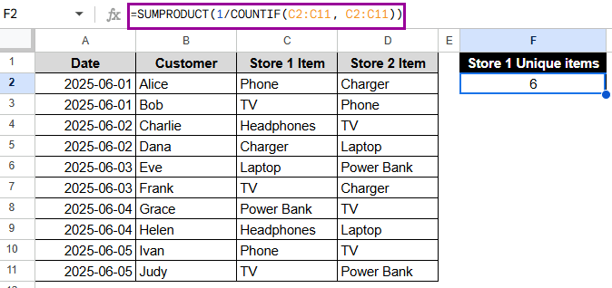
Note:
This method is simple if you’re working with big datasets or need a formula without helper columns.
Combining FLATTEN and COUNTUNIQUE Functions to Find Unique Values
Users can easily find the total number of unique values when data is spread out across multiple columns. The FLATTEN function helps by putting all the values from these columns into one column. This allows the COUNTUNIQUE function to identify unique entries across all of these columns.
Now, the method will tell us how many different products are involved in Store 1 and Store 2.
Steps:
➤ Choose a blank cell, F2.
➤ Enter the formula:
=COUNTUNIQUE(FLATTEN(C2:D11))
➤ Hit Enter to get the result. There are 6 different products in these stores.
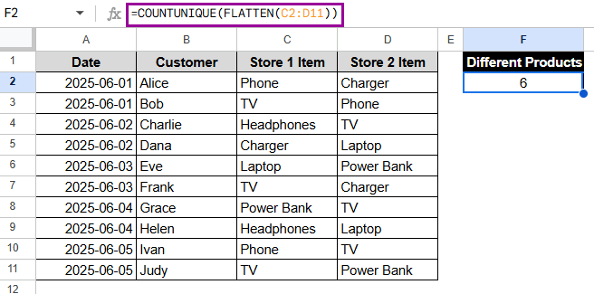
Note:
This function combines columns into one before counting. It works with both numbers and text.
Frequently Asked Questions
How do I count unique values in a Google Sheets column?
You can find out how many unique values are in a single column by using =COUNTUNIQUE(range) or =COUNTA(UNIQUE(range)). Both functions automatically ignore duplicates and only return the total number of unique entries.
Can I count unique values based on multiple conditions?
Yes. You can use the FILTER function with UNIQUE and then put everything in COUNTA to count how many entries meet all of the criteria while still being unique.
What if I want to count unique values across multiple columns?
Before checking for uniqueness, try merging values into a single list with =COUNTUNIQUE(FLATTEN(range1, range2)). This is useful when your data is spread out horizontally across multiple fields or categories.
Are empty cells counted as unique values?
No, the UNIQUE and COUNTUNIQUE functions both skip cells that are blank or empty. So, the count only includes entries that are not empty and are truly unique.
Concluding Words
For data analysis, cleanup, and reporting, it’s important to count unique values. Google Sheets has many different tools, from simple one-line formulas to complicated filters that can handle multiple criteria. Choose the method that fits your needs and the structure of your data, and use it with confidence.