When using the IMPORTRANGE function in Google Sheets to pull data from another spreadsheet, you might occasionally run into the frustrating “Error loading data” message. This can break workflows and affect dashboards or summaries that depend on live data imports.
This article will guide you through what causes the error, how to fix it, and provide step-by-step instructions and best practices to ensure IMPORTRANGE works reliably.
Steps to use the IMPORTRANGE function correctly and avoid the “error loading data” message in Google Sheets:
➤ Use this formula structure as a starting point:
=IMPORTRANGE(“https://docs.google.com/spreadsheets/d/12345abcdXYZ/edit”, “Product Data!A1:B4”)
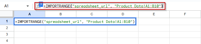
➤ Make sure the sheet name (“Product Data”) exactly matches the tab name in the source spreadsheet, including spaces and capitalization
➤ The range (A1:B4) must be within the actual data range of the source sheet
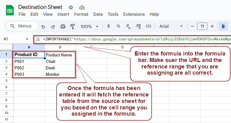
➤ After entering the formula, click “Allow Access” to authorize the data connection
➤ Begin with a small, valid range to test before expanding the formula to larger ranges or different sheets
Use the Correct Sheet Name and Range
A frequent cause of the “error loading data” message is referencing a sheet name that doesn’t exist or a range that’s invalid. Even a small typo in the sheet name or an incorrect cell range will break the formula.
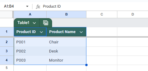
These are the datasets that we will be using to demonstrate the method:
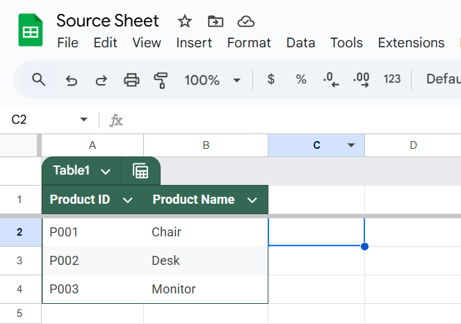
Source Sheet:
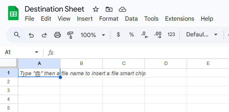
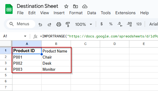
Destination Sheet:
Steps:
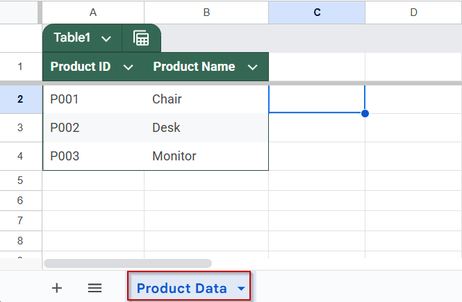
➤ Open the source spreadsheet and confirm the exact name of the sheet tab (e.g., Product Data)
➤ In your IMPORTRANGE formula, make sure the sheet name matches exactly, including spaces and capitalization
➤ Use this correct format:
=IMPORTRANGE(“spreadsheet_url”, “Product Data!A1:B4”)
➤ Do not use something like productdata!A1:B4, this will trigger the “error loading data” issue
Confirm That the Range Exists in the Source File
One of the most overlooked causes of the “Google Sheets IMPORTRANGE error loading data” is referencing a range that doesn’t exist in the source spreadsheet. If your formula tries to pull in cells beyond the actual data, Google Sheets will fail to load anything. This method helps you verify and correct the range to ensure that data can be successfully imported.
Steps:
➤ Open the source spreadsheet
➤ Navigate to the sheet you’re referencing and examine how many rows and columns are filled with data.
➤ Double-check that your formula’s range (e.g., A1:B4) is within the actual data bounds
➤ Try using a smaller, safe test range like:
=IMPORTRANGE(“spreadsheet_url”, “Product Data!A1:B3”)
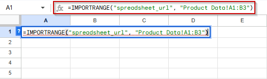
➤ Avoid referencing large or unused ranges like A1000:B2000, unless you’re certain those cells contain data
Grant Access to the Source Spreadsheet
If you haven’t granted permission to connect the two spreadsheets, Google Sheets will not be able to import any data. This is one of the most common reasons for the “Google Sheets IMPORTRANGE error loading data” message. Without proper access, even a perfectly written formula will fail.
Steps:
➤ After entering your formula, you’ll see an “Allow Access” button
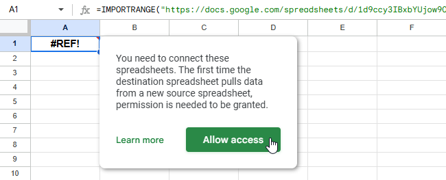
➤ Click the button to authorize the data connection between the spreadsheets
➤ If no prompt appears, open the source spreadsheet manually using the URL from your formula
➤ Click “Request access” if you do not already have it

➤ Once access is granted, return to the destination spreadsheet
➤ The data should now load automatically without error
Always Use the Correct Spreadsheet URL Format
Using a partial or malformed link will cause the IMPORTRANGE function to fail with a “loading data” error. Check the method below for the correct way of using the spreadsheet URL.
Steps:
➤ Copy the full URL from the browser address bar of the source file
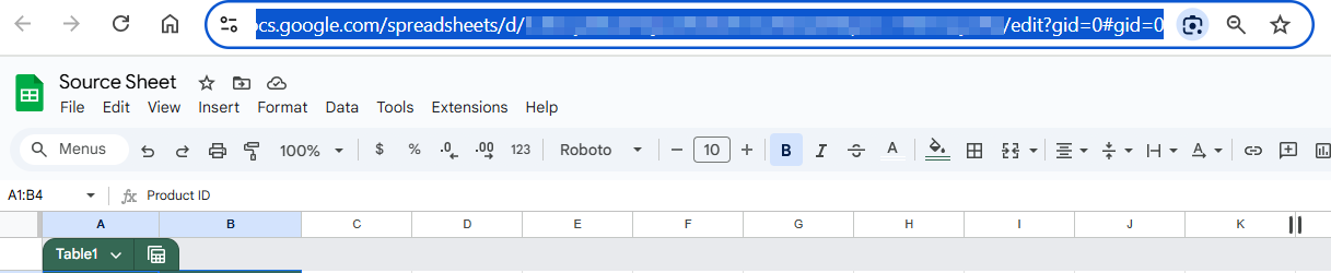
➤ The URL should look like this:
https://docs.google.com/spreadsheets/d/1aBcDeFgHiJkLmNoPqRsTuVwXyZ1234567890/edit
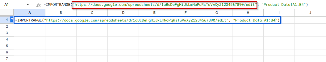
➤ Use it in your formula like this:
=IMPORTRANGE(“https://docs.google.com/spreadsheets/d/1aBcDeFgHiJkLmNoPqRsTuVwXyZ1234567890/edit”, “Product Data!A1:B3”)
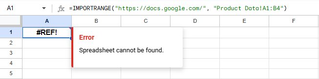
➤ Do not use a shortened or incomplete link (like https://docs.google.com), or your formula will fail
Example of a Working IMPORTRANGE Formula
Here’s a working example you can test to validate that your connection and syntax are correct, follow this and you should not get any errors.
=IMPORTRANGE(“https://docs.google.com/spreadsheets/d/12345abcdXYZ/edit”, “Product Data!A1:B4”)
➤ The URL must be valid and accessible
➤ The sheet name must match exactly
➤ The range must exist and contain data
➤ Access must be granted between the two files
➤ Once entered, the IMPORTRANGE function will fetch the data from the source sheet for you.
Frequently Asked Questions
Can I fix this error if the files are owned by different Google accounts?
Yes. You just need to make sure your current Google account has viewing access to the source spreadsheet. Without access, IMPORTRANGE will not load any data.
Does the error go away automatically after access is granted?
Yes. Once you allow access or the file owner shares it with you, the “error loading data” message should disappear on its own.
Can IMPORTRANGE work with named ranges instead of A1 notation?
Yes, but the named range must be created in the source sheet, and you must reference it by exact name, no quotes or exclamation points.
What if my data isn’t loading even after fixing everything?
Try using a simpler range like A1:B2 to test. If that works, the issue may be related to the amount of data you’re trying to import or a temporary issue with Google Sheets itself.
Wrapping Up
If you’re seeing a “Google Sheets IMPORTRANGE error loading data”, the issue is almost always due to one of the following: incorrect sheet name, invalid range, missing file access, or a malformed URL. By carefully reviewing each part of your formula and following the steps above, you can quickly resolve the problem and resume working with live, linked data across spreadsheets.