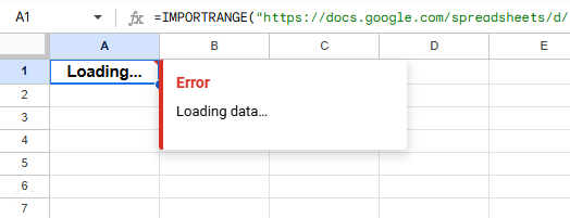
If you see an “Internal error” while using the IMPORTRANGE function in Google Sheets, you’re not alone. This cryptic error usually appears when something goes wrong behind the scenes, whether it’s with Google’s servers, the spreadsheet link, or access permissions.
This article walks you through the most common reasons why you get the “internal error” and offers step-by-step solutions to fix it.
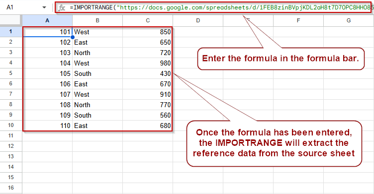
Steps to use IMPORTRANGE function correctly in Google Sheets:
➤ Use this formula structure as a starting point:
=IMPORTRANGE(“https://docs.google.com/spreadsheets/d/abcd1234XYZ/edit”, “Sales Data!A2:C11”)
➤ Make sure the URL is a clean, full link and not shortened or redirected
➤ Ensure the sheet name (“Sales Data”) and range (A2:C11) exist and are spelled exactly as in the source
➤ After entering the formula, click “Allow Access” if prompted
➤ Always test the base formula first before combining it with functions like QUERY or FILTER
Granting Access to Fix IMPORTRANGE Internal Errors
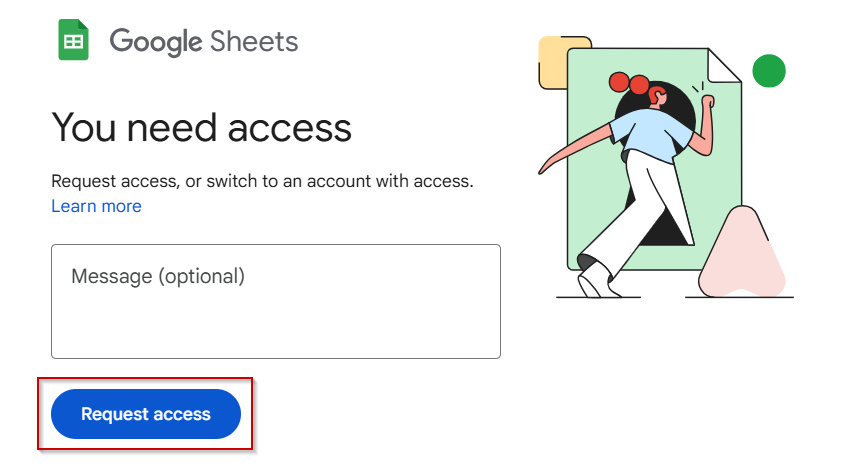
One of the most common causes of the IMPORTRANGE “internal error” is failing to grant permission between the source and destination spreadsheets. Without this authorization, Google Sheets cannot retrieve data, even if the formula is written correctly. This method shows you how to resolve the error by manually allowing access.
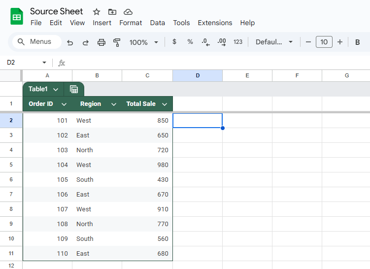
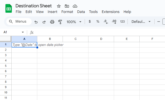
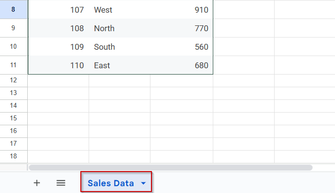
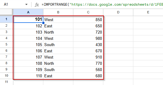
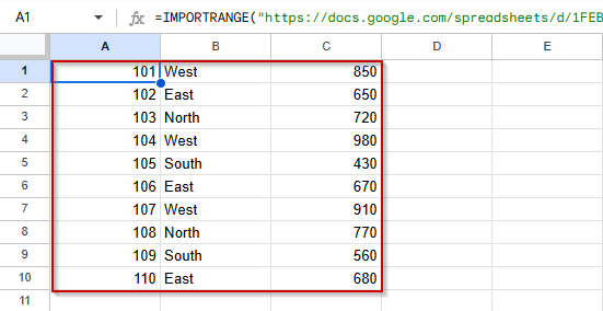
These are the datasets we will be using for this article:
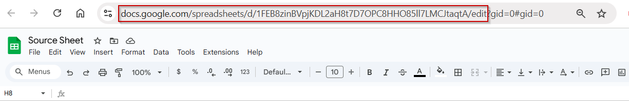
Source Sheet:
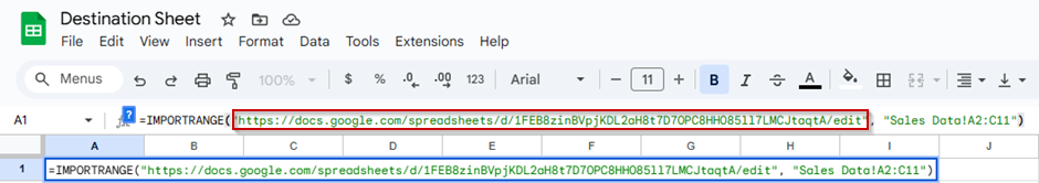
Destination Sheet:
Steps:
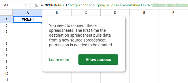
➤ Enter your IMPORTRANGE formula in the destination sheet:
=IMPORTRANGE(“https://docs.google.com/spreadsheets/d/abcd1234XYZ/edit”, “Sales Data!A2:C11”)
➤ If it shows a #REF! error, click the cell, then click “Allow Access” when prompted.
➤ If the access prompt doesn’t appear, try pasting the formula into a new cell or a different sheet tab.
➤ Double-check that you’re logged into a Google account with access to both spreadsheets.
➤ If you are still not able to get access then check your source sheet. If it is owned by someone else request for access from them.
Resolve Internal Errors by Fixing Sheet Name or Range Reference
Another common cause of the IMPORTRANGE internal error is a mismatch between the sheet name or cell range specified in your formula and the actual content in the source spreadsheet. This method helps you fix the issue by verifying and correcting these references.
Steps:
➤ Double-check that the sheet name in your formula exactly matches the name of the tab in the source file, including capitalization, spacing, and punctuation.
For example, “Sales Data” is not the same as “sales data”.
➤ Make sure the cell range exists. If your formula refers to “Sales Data!A2:C11” but the source sheet only contains rows up to 5, the formula may return an internal error.
➤ Example of a correct formula:
=IMPORTRANGE(“https://docs.google.com/spreadsheets/d/abcd1234XYZ/edit”, “Sales Data!A2:C11”)
Avoid Internal Errors by Using the Correct Spreadsheet URL
An often-overlooked cause of the IMPORTRANGE internal error is using an invalid or modified link. The formula requires the full, clean URL of the source spreadsheet, not a form URL, preview link, or a shortened version of it. This method helps ensure your URL is formatted correctly so that the IMPORTRANGE function can connect without issues.
Steps:
➤ Use the full Google Sheets URL format:
https://docs.google.com/spreadsheets/d/abcd1234XYZ/edit
➤ Remove any extra parts after /edit, such as ?usp=sharing, &pli=1, etc.
➤ Avoid using links that contain /viewform, /preview, URL shorteners (like bit.ly or goo.gl).
Using the proper raw spreadsheet link ensures a reliable connection and prevents internal errors from blocking your data import.
Prevent Internal Errors by Testing IMPORTRANGE Before Nesting
IMPORTRANGE can sometimes cause internal errors when used within other functions, such as QUERY or FILTER, before the data has fully loaded. This method helps you avoid such mistakes by first confirming the data connection works independently, then gradually adding more complex formulas.
Steps:
➤ Begin with a simple IMPORTRANGE formula to ensure data loads correctly:
=IMPORTRANGE(“https://docs.google.com/spreadsheets/d/abcd1234XYZ/edit”, “Sales Data!A2:C11”)
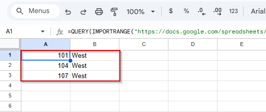
➤ Once data appears without errors, safely wrap it inside other functions such as QUERY:
=QUERY(IMPORTRANGE(“https://docs.google.com/spreadsheets/d/abcd1234XYZ/edit”, “Sales Data!A2:C11”), “SELECT Col1, Col2 WHERE Col2=’West'”)
➤ Avoid nesting too early; confirm each step works before combining formulas to prevent internal errors.
Frequently Asked Questions
Why do I get an internal error when using IMPORTRANGE?
It usually occurs due to missing authorization, incorrect sheet names or ranges, invalid URLs, or nesting IMPORTRANGE in formulas before the data loads properly.
How do I fix the #REF! error with IMPORTRANGE?
Click the cell showing #REF!, then click “Allow Access” to authorize the connection between spreadsheets. Make sure you’re logged into the correct Google account.
Can IMPORTRANGE cause errors if sheet names change?
Yes, any change in sheet tab names or range references causes errors. Always verify the exact sheet name and that the range exists before using IMPORTRANGE.
Is it okay to nest IMPORTRANGE inside QUERY or FILTER?
Yes, but only after the basic IMPORTRANGE formula works. Nesting too early may cause internal errors. Always test IMPORTRANGE alone first before combining it with other functions.
Wrapping Up
The IMPORTRANGE function is a powerful way to connect data across spreadsheets, but internal errors can occur if access isn’t authorized, ranges are incorrect, or the formula is misused. By carefully checking your URL, confirming sheet names and ranges, and allowing access when prompted, you can resolve most issues quickly. Always test the base IMPORTRANGE formula first before combining it with other functions like QUERY or FILTER. With the right setup, you’ll ensure smooth, error-free data imports every time.