Combining data from multiple sheets into one summary table is a common requirement when working with reports, monthly logs, or team data. The QUERY function in Google Sheets is an excellent way to filter and analyze information using SQL-like statements.
However, QUERY doesn’t directly allow selecting from multiple sheets unless you combine them first. In this article, you’ll learn how to use Google Sheets QUERY across multiple sheets using clean formulas and efficient structures that update automatically.
Steps to use Google Sheets QUERY across multiple sheets:
➤ Open your central Google Sheet (e.g., “Summary“).
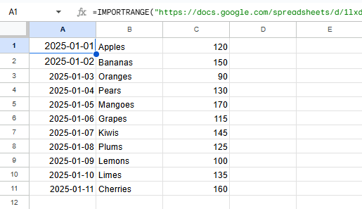
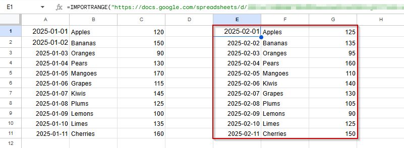
➤ In an empty sheet, use this formula to import January’s data:
=IMPORTRANGE(“<URL of January file>”, “JanuarySales!A2:C12”)
➤ In a separate range (e.g., starting at E2), import February’s data:
=IMPORTRANGE(“<URL of February file>”, “FebruarySales!A2:C12”)
➤ Click “Allow Access” if prompted for either file.
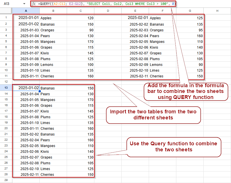
➤ Once both datasets are imported, use this formula in A13 to merge and filter:
=QUERY({A2:C12; E2:G12}, “SELECT Col1, Col2, Col3 WHERE Col3 > 100”, 0)
IMPORTRANGE with QUERY Function to Query Across Sheets in Different Files
If your data lives in separate Google Sheets files instead of different tabs in one file, the IMPORTRANGE function allows you to bring that data into a central sheet. This method is helpful when working with distributed teams or data stored in separate spreadsheets.
You’ll need to import the range from each external sheet first, then apply the QUERY formula on the combined result.
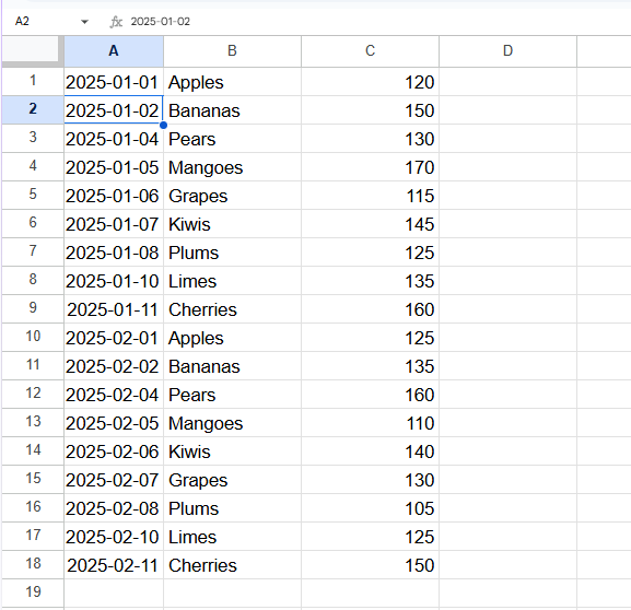
These are the datasets that we will be using for this article:
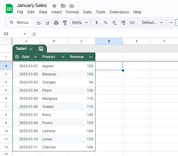
January Sales:
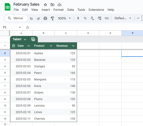
February Sales:
Steps:
➤ Open the Google Sheet where you want to combine the data.
➤ In a new sheet, enter this formula to import data from the first external sheet:
=IMPORTRANGE(“<URL of January file>”, “JanuarySales!A2:C12”)
➤ Repeat this for the second file in another range:
=IMPORTRANGE(“<URL of February file>”, “FebruarySales!A2:C12”)
➤ Grant permission if prompted.
➤ Now use the QUERY function like this in A13 (assuming imported data is in ranges A2:C12 and E2:G12:
=QUERY({A2:C12; E2:G12}, “SELECT Col1, Col2, Col3 WHERE Col3 > 100”, 0)
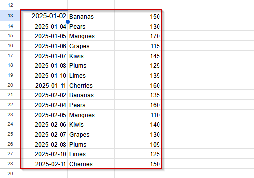
This merges and filters the data from both remote sheets.
Combine and Filter Data from Multiple Tabs in the Same Google Sheets File
The simplest and most reliable way to query multiple sheets in Google Sheets is by combining the data from those sheets using the {} array syntax. Then, apply a QUERY function to this combined dataset. This method is perfect when your sheets share the same structure.
For example, let’s say you’re tracking monthly sales and have two tabs named JanuarySales and FebruarySales. Each tab contains three columns: Date, Product, and Revenue. The datasets used for January Sales and February Sales are the same as before.
Steps:
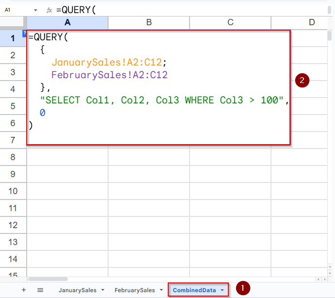
➤ Go to a new sheet (e.g., “CombinedData“) where you want the merged output.
➤ Click on cell A1 and enter the following formula:
=QUERY(
  {
    JanuarySales!A2:C12;
    FebruarySales!A2:C12
  },
  "SELECT Col1, Col2, Col3 WHERE Col3 > 100",
  0
)
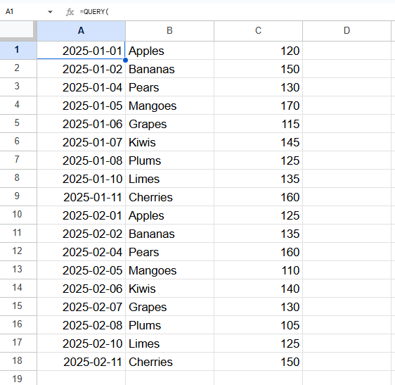
➤ Press Enter.
➤ You’ll now see all rows from both sheets where the revenue is greater than 100.
Note:
Col1, Col2, and Col3 refer to the first, second, and third columns in the combined array (Date, Product, Revenue). Adjust your WHERE clause as needed.
Using INDIRECT Function for Dynamic Sheet References in Google Sheets
If you want more flexibility in referencing multiple sheets, especially when the sheet names change often or are generated dynamically, the INDIRECT function can help. While it’s limited to pulling data within the same spreadsheet, it lets you reference sheet names based on cell values, dropdowns, or formulas. This is especially helpful for automating reports across many tabs like “JanuarySales“, “FebruarySales“, and so on.
One important thing to note is that INDIRECT does not update automatically if you rename your sheets, and it doesn’t work across separate Google Sheets files. Still, when used right, it allows you to keep your QUERY formula clean and responsive to changes in sheet structure.
Steps:
➤ Go to the sheet where you want to aggregate the data (e.g., a new sheet named “Summary“).
➤ Click on cell A1.
➤ Paste the following formula:
=QUERY({
INDIRECT(“JanuarySales!A2:C”);
INDIRECT(“FebruarySales!A2:C”)
}, “SELECT Col1, Col2, Col3 WHERE Col3 > 100”, 0)
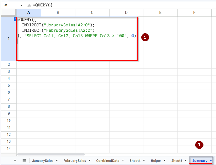
➤ Press Enter.
➤ Your Summary sheet will now show all rows from both monthly sheets where the Revenue column (Col3) is greater than 100.
Note:
You can use INDIRECT(A1 & “!A2:C”) to dynamically reference a single sheet, where cell A1 contains the sheet name (like JanuarySales). This lets you query different sheets without rewriting the formula each time. However, INDIRECT does not work inside array literals (i.e., {}) for combining multiple sheets into one query. For merging data from multiple tabs, use direct references like {Sheet1!A2:C; Sheet2!A2:C} instead.
Frequently Asked Questions
Can I use QUERY on multiple sheets with different column layouts?
No. All sheets you merge using {} must have the same number of columns and the same order of fields. Otherwise, the merged array will return a formula error or unexpected results. To avoid errors, clean and align your sheets before querying.
Will the QUERY update automatically when I add new rows?
Yes, as long as you reference dynamic ranges like A2:C (instead of A2:C100), your merged data will automatically include new rows. The QUERY will update its results without needing to adjust the formula.
Can I use QUERY across three or more sheets?
Absolutely. Just keep stacking the sheets with semicolons inside curly braces. For example:
=QUERY({Sheet1!A2:C; Sheet2!A2:C; Sheet3!A2:C}, “select Col1, Col3 where Col3 > 100”, 0)
Just make sure all sheets follow the same column structure.
What happens if one of the sheets is empty?
If any of the referenced ranges are empty, Google Sheets will simply ignore them in the output. The QUERY will run normally and show only rows from sheets that contain data. There’s no error unless all sources are empty.
Can I combine QUERY with other functions like SORT or FILTER?
Yes. QUERY works well with SORT, UNIQUE, and FILTER. You can even wrap your entire QUERY formula inside SORT() to order the output by any column you want. This makes it ideal for dashboards and reports.
Wrapping Up
Although Google Sheets doesn’t support querying multiple sheets natively in one function, you can merge sheets using array notation ({}) or external functions like IMPORTRANGE() and INDIRECT() to achieve the same result. With a solid understanding of how to align your datasets and write flexible queries, you can summarize information across months, teams, or files without tedious manual copying.