When working with datasets in Google Sheets, you may want to sum values only if another column is not blank. For example, you might want to sum amounts only where a corresponding status or name exists.
Google Sheets doesn’t have a direct SUMIF(…, IS NOT BLANK) function, but you can use a smart condition, such as “<>”, to effectively exclude blank cells. In this article, we will guide you through the process step by step.
Steps to use SUMIF to ignore blank cells in another column in Google Sheets
➤ Use this method to sum values only when corresponding cells (e.g., Status) are not blank.
➤ Select a blank cell where you want the result (e.g., D2).
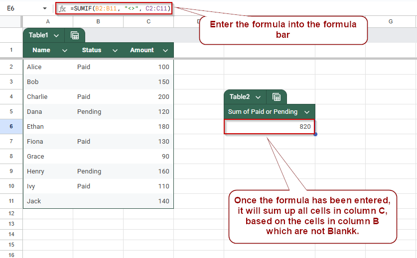
➤ Enter the formula: =SUMIF(B2:B11, “<>”, C2:C11)
➤ B2:B11 is the range where you’re checking for non-blank values (e.g., Status).
➤ “<>” is the condition that filters out blank cells.
➤ C2:C11 is the range of numeric values (e.g., Amount) to sum.
➤ Press Enter to get the sum of only those rows where the Status is filled.
Use SUMIF Ignoring Blank Cells in Another Column in Google Sheets
When working with data in Google Sheets, you may often want to calculate totals only if specific cells contain values, like summing payments only when a status is recorded. The SUMIF function is perfect for this. By checking whether a corresponding cell is not blank, you can ensure your totals reflect only complete or relevant entries.
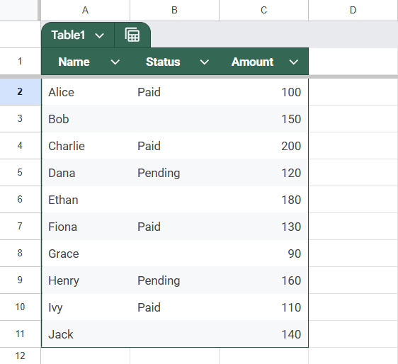
This is the dataset we will be using to demonstrate the methods:
Steps:
➤ Click on a blank cell where you want the result.
➤ Enter the formula:
=SUMIF(B2:B11, “<>”, C2:C11)
![]()
➧ <> tells Google Sheets to ignore blanks
➧ C2:C11 is the range of values to sum
➤ Press Enter.
![]()
The formula will sum only the Amounts where the Status is not blank (i.e., where there’s a value in column B).
Combine FILTER and SUM for More Flexibility While Ignoring Blank Cells
If you need more control than SUMIF offers, such as checking multiple conditions or dynamically referencing ranges, you can combine FILTER with SUM. This approach is great when you want to sum a column only if another column is not blank, but also want the flexibility to expand the logic.
Steps:
➤ Click on a blank cell where you want the result.
➤ Enter the formula:
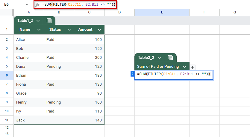
=SUM(FILTER(A2:A11, B2:B11 <> “”))
➤ Press Enter
![]()
This formula sums values from column A only where the corresponding cell in column B is not empty. Unlike SUMIF, FILTER lets you build more complex conditions and reference ranges dynamically.
SUMPRODUCT Function to Sum Truly Non-Empty Cells
Sometimes cells look blank but actually contain invisible spaces, which can lead to incorrect totals when using basic functions like SUMIF. These space-filled cells trick SUMIF into including them in calculations, even though they shouldn’t count as valid entries.
To solve this, we can combine the SUMPRODUCT, LEN, and TRIM functions to accurately identify and sum rows where the corresponding cells are truly non-empty, even when hidden characters exist. This method ensures your total reflects only meaningful data.
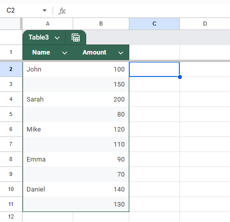
We will be using this dataset to demonstrate this method. In this dataset, some cells contain spaces, technically making them non-blank cells.
Steps:
➤ Click on a blank cell where you want the sum to appear.
➤ Enter the formula:
=SUMPRODUCT(–(LEN(TRIM(A2:A11))>0), B2:B11)
![]()
➤ Press Enter.
![]()
Frequently Asked Questions
How do I sum values only if another cell isn’t blank?
Use =SUMIF(B2:B11, “<>”, A2:A11). It adds values from Column A only when the corresponding cell in Column B is not empty.
Can I sum cells based on multiple non-blank columns?
Yes. Use =SUM(FILTER(A2:A11, (B2:B11<>””) * (C2:C11<>””))) to include rows where both Column B and Column C are not blank.
What if I want to ignore zeros as well as blanks?
Use =SUM(FILTER(A2:A11, (B2:B11<>””) * (A2:A11<>0))). This filters out both blank and zero-value rows before summing Column A.
Can I use SUMIFS instead of SUMIF?
Yes, SUMIFS supports multiple conditions. Example: =SUMIFS(A2:A11, B2:B11, “<>”) lets you sum Column A only when Column B is not blank.
Wrapping Up
Summing values in Google Sheets while ignoring blank cells is a common task when working with structured data. Whether you’re tracking sales, attendance, or any conditional totals, using SUMIF or FILTER functions allows you to keep your results accurate and meaningful. SUMIF is perfect for straightforward conditions, while FILTER offers flexibility for multiple criteria. By mastering these methods, you ensure your spreadsheets reflect only the data that matters, skipping over empty cells and focusing on what’s important.