
In Google Sheets, users often need to add up numbers based on whether a related cell has certain text in it. When you are working with descriptive datasets and need to filter or combine values based on matching certain words or parts of strings in another column, this challenge usually comes up. Using SUMIF in Google Sheets when another cell contains text makes it much easier to handle data like tracking performance, managing inventory, or just analyzing products.
To add up values in Google Sheets based on whether a different cell has certain text, do the following steps:
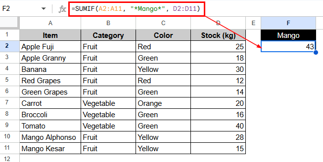
➤ Select the cell where you want to return the sum, in this case, F2.
➤ Enter the formula using this structure:
=SUMIF(A2:A11, “*Mango*”, D2:D11)
➤ Press Enter to calculate the total based on the match
This article will show you several ways to add up values in Google Sheets based on the text in another cell. We will show you how to use SUMIF (with both partial and exact matches), SUMIFS (for multiple criteria), FILTER with SUM, and array formulas like ARRAYFORMULA with SEARCH.
Using SUMIF with Partial Text Match
You can use the SUMIF function to add numbers that meet a certain condition. When you work with text, you can use wildcards like asterisks (*) to find matches for parts of the text. You need to change the range to point to the cells that have the text condition. You can set sum_range to be the column that has the numbers you want to add up.
Let’s say, here, the dataset has a list of fruits and vegetables that a grocery store sells, along with their names, categories, colors, and stock levels.
Steps:
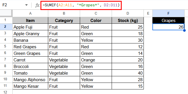
➤ Select the cell where you want the result (e.g. F2).
➤ Enter the formula using this structure:
=SUMIF(A2:A11, “*Grapes*”, D2:D11)
➤ Press Enter to calculate the total “Grapes” based on the match
Note:
The asterisk * can stand in for any number of characters. This formula is not case-sensitive.
Using SUMIF with Exact Text Match
To only add up values when a cell has the exact text you’re looking for, take the wildcards out of the criteria. In this case, only rows with text that exactly matches the total are counted, so there is no chance of including similar or partial entries by mistake.
Steps:
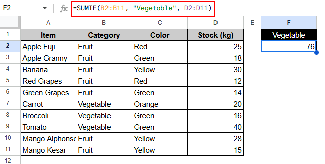
➤ Let’s say, the target cell is F2.
➤ Type the formula:
=SUMIF(B2:B11, “Vegetable”, D2:D11)
➤ Press Enter to calculate the total stock for items exactly categorized as “Vegetable.”
Note:
This method of summing rows only works when the condition cell’s text is an exact match. It works best with datasets that are structured or categorized.
Using SUMIFS for Multiple Conditions
The SUMIFS function lets you use more than one condition. For example, you can add up values when a cell has certain text and another cell meets a date or number condition. You can also use text-based criteria along with numeric thresholds or date comparisons to get the exact data you want, such as only adding up green fruits sold after a certain date.
Steps:
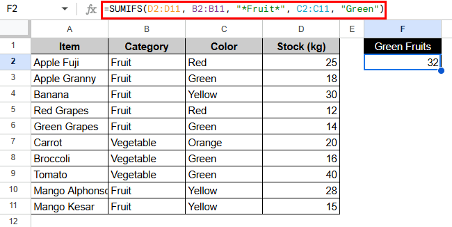
➤ Select your output cell, such as F2.
➤ Use the following structure in your formula:
=SUMIFS(D2:D11, B2:B11, “*Fruit*”, C2:C11, “Green”)
➤ Press Enter to apply both filters.
Note:
This method is useful if you need to improve your summing logic. Wildcards can only be used for conditions that are based on text.
Alternatives to SUMIF & SUMIFS
You can use functions like FILTER with SUM or ARRAYFORMULA with SEARCH instead of SUMIF and SUMIFS to get more flexible and dynamic conditions. When you have partial matches or more than one criterion, these methods give you more control.
Using FILTER with SUM for Flexible Matching
You can use the FILTER function with SUM to add up values based on complex or partial text matches in a dynamic way. You can use functions like SEARCH or REGEXMATCH inside FILTER to only include rows that meet your text criteria and then add up the values that come out.
Steps:
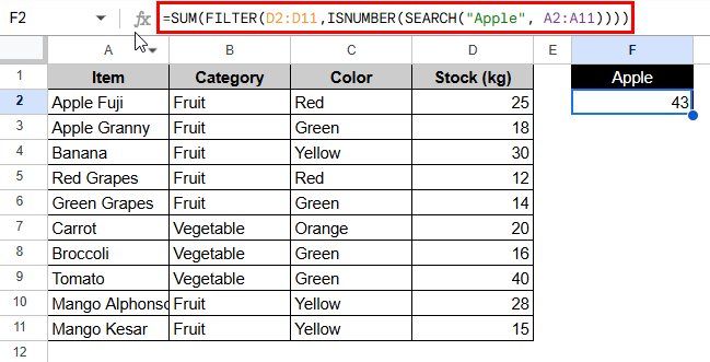
➤ Select the result cell, F2.
➤ Now enter:
=SUM(FILTER(D2:D11,ISNUMBER(SEARCH(“Apple”, A2:A11))))
➤ Hit Enter to calculate the sum of “Apple”.
Note:
This formula lets you match parts of strings without caring about the case. It’s helpful when text is part of longer strings or mixed with other words.
Using ARRAYFORMULA for Advanced Text Filtering
ARRAYFORMULA function lets you work with whole ranges at once, and it’s especially useful for more complicated logic with SEARCH. It also lets you make one formula that checks every cell in your text range and gives you an array of results. This means you don’t have to drag formulas down or make helper columns.
Steps:
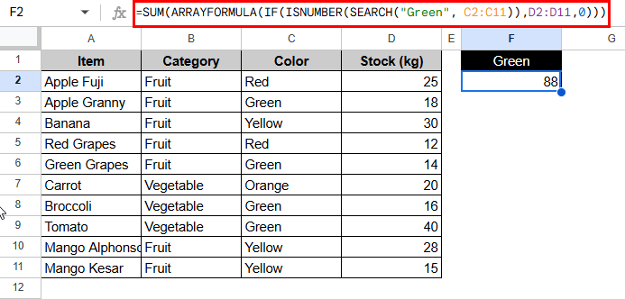
➤ Click the output cell, F2.
➤ Type the following formula into a cell:
=SUM(ARRAYFORMULA(IF(ISNUMBER(SEARCH(“Green”, C2:C11)),D2:D11,0)))
➤ Click Enter to get the sum of all Green fruits and vegetables.
Note:
Use it when you have dynamic data and other functions can’t handle your logic. Similar to FILTER, it allows you to customize the return values.
Frequently Asked Questions
In Google Sheets, what’s the difference between SUMIF and SUMIFS?
SUMIF only works with one condition, but SUMIFS can work with more than one. If you only have one condition, use SUMIF. If you need to combine two or more logical filters, use SUMIFS.
Is it possible to use SUMIF with “contains” logic?
Yes, you can use wildcards like * to see if a cell has a word or part of a word:
=SUMIF(range, “*word*”, sum_range)
Is SUMIF case-sensitive in Google Sheets?
No, SUMIF isn’t sensitive about cases When it matches the text, it doesn’t care if the letters are uppercase or lowercase.
How do I add up values if there is more than one keyword in another cell?
You need to use ARRAYFORMULA or FILTER with SEARCH or REGEXMATCH to match more than one keyword. The standard SUMIF function does not allow the use of OR logic with multiple substrings.
What happens if the criteria range cell is empty?
If the cell is empty and you use SUMIF or SEARCH, the condition won’t be met, and that row won’t be included in the total.
Can I sum values based on a text that appears at the start or end of a string?
Yes. In SUMIF, you can use wildcards like “text*” to match the start of a string or “*text” to match the end of a string.
Concluding Words
In conclusion, the SUMIF function in Google Sheets with text-based conditions gives you a lot of control over your data. These methods let you summarize your data in Google Sheets based on text conditions in a way that is both flexible and powerful. By learning how to use these functions, you can automate complicated calculations, cut down on mistakes, and keep your google sheets consistent.