[Fixed] VLOOKUP Not Working in Google Sheets: 4 Cases

If your VLOOKUP formula in Google Sheets isn’t returning the right result, or any result at all, you’re not alone. This function is powerful but easy to misconfigure. Whether it’s due to incorrect ranges, mismatched data types, or missing exact matches, identifying the root cause will help you get it working again.

This article explains the most common reasons VLOOKUP fails and shows you how to troubleshoot and fix each issue effectively.

One of the most frustrating issues with the VLOOKUP function in Google Sheets is when it returns the #N/A error. This usually means that your lookup value wasn’t found in the search range, even when it appears to be present. Common causes include extra spaces, inconsistent formatting, or incorrect range setup.

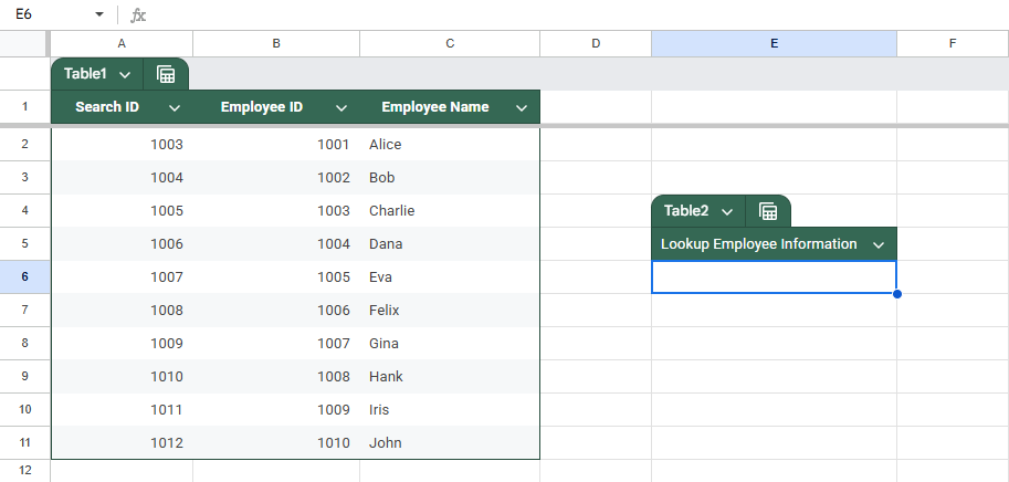
This is the dataset we will be using to demonstrate the methods:

Steps:

➤ Ensure the lookup value is in the first column of the range. In our case, we are using “Search ID” as our lookup column.

In this case, we are trying to look up from column A, but the range we have assigned starts from column B. Therefore, a #N/A error is triggered.

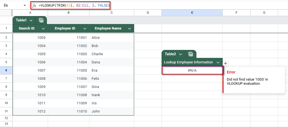
➤ Double-check for typos, trailing spaces, or different capitalizations.
➤ Use this formula to clean lookup values using the TRIM function in case there are any hidden characters:

Sometimes, your VLOOKUP formula doesn’t return the exact match you expect. Instead, it shows a seemingly random or incorrect value. This usually happens because the range_lookup argument (the fourth argument in VLOOKUP) is either omitted or explicitly set to TRUE.

When range_lookup is set to TRUE (or omitted altogether), VLOOKUP tries to find an approximate match. This means it will return the closest value that is less than or equal to your search term, which can lead to unexpected results, especially if your data isn’t sorted in ascending order.

Steps:

To ensure VLOOKUP always returns the exact match:

➤ Use FALSE as the fourth argument:

This tells Google Sheets to find only an exact match.

Sometimes, your lookup value looks correct, but VLOOKUP still returns #N/A. This usually occurs because of hidden characters, such as line breaks, non-breaking spaces, or inconsistent data formatting (e.g., numbers stored as text in one place and as actual numbers in another). These minor differences can disrupt your formula, even when the values appear identical.

Steps:

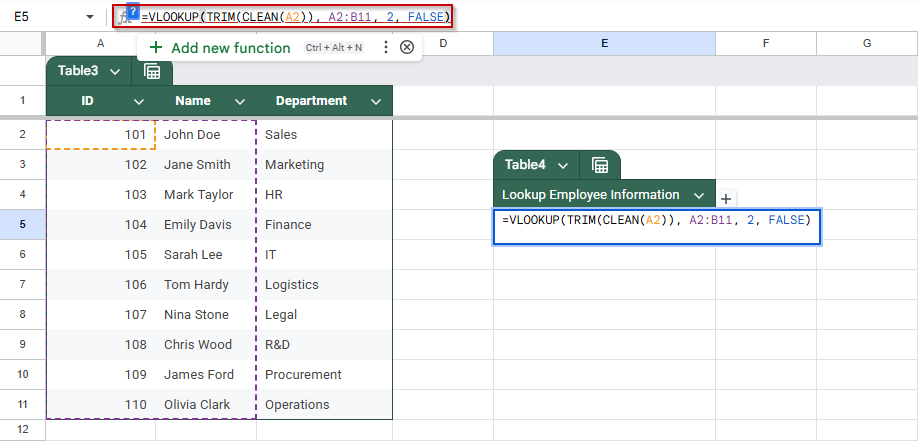
➤ Clean the lookup value using TRIM and CLEAN to remove hidden characters and extra spaces:

➤ Clean the entire data column (optional but recommended) using ARRAYFORMULA with TRIM and CLEAN. This helps if your source data also has formatting issues:

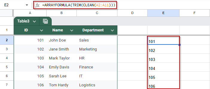
Paste the result into a helper column and point your VLOOKUP formula to this cleaned-up range for better accuracy.

VLOOKUP will return an error if the column index number you provide is greater than the number of columns in your lookup range. The column index tells VLOOKUP which column’s value to return, based on where your lookup range starts. If this number is too high, pointing to a column that doesn’t exist in your specified range, Google Sheets can’t find the valu,e and the formula breaks.

Steps:

➤ Count the columns in your range, starting from the leftmost column in the range as 1.

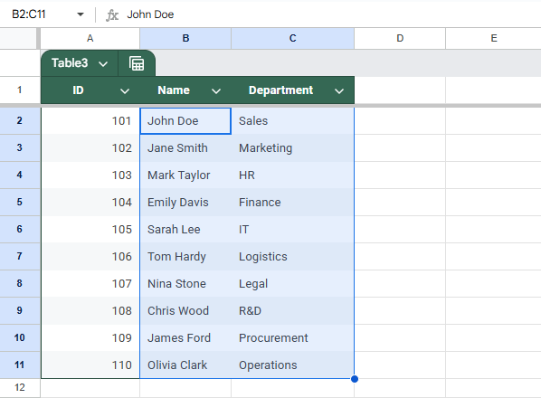
If your range is B2:C11, then B is column 1 and C is column 2. So, the maximum column index number you can use here is 2

➤ Make sure the column index number doesn’t exceed the number of columns in the range. Using 3 in a B2:C11 range will cause an error.

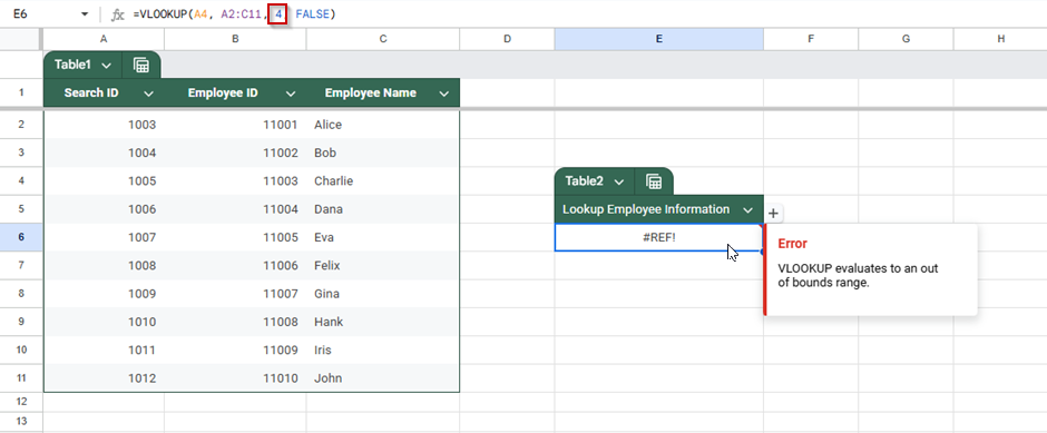
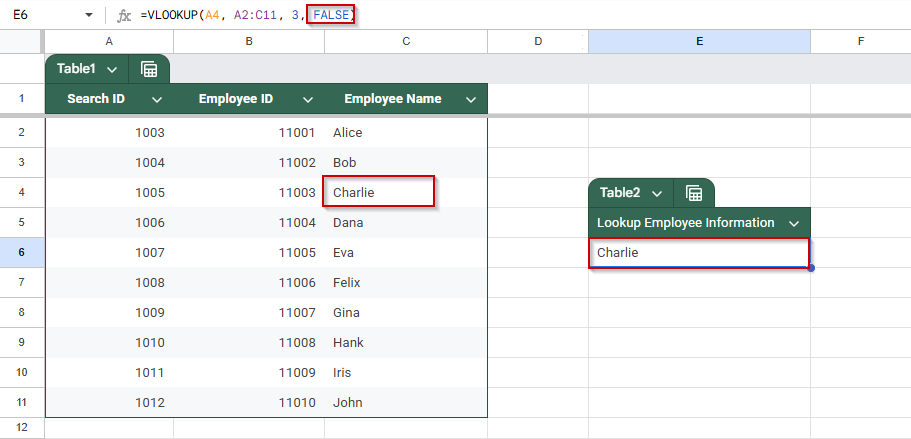
➤ Adjust the column index based on your lookup goal. If your search value is in column A and you want to return a name from column C, your range must include all three columns (A to C), and the column index should reflect the relative position:

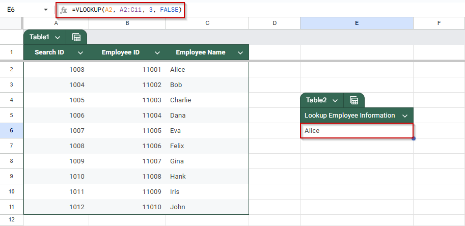
Here, A is column 1 in the range, and C is column 3. So, index 3 is valid and returns the name correctly

Frequently Asked Questions

Why does VLOOKUP return #N/A even when the value is present?

It could be due to leading/trailing spaces, text vs number mismatch, or the value not being in the first column of the range.

How do I make VLOOKUP case-insensitive?

VLOOKUP is case-insensitive by default. Use EXACT + FILTER if you need case-sensitive lookups.

Can VLOOKUP search from right to left?

No. Use INDEX + MATCH or XLOOKUP (if available) for right-to-left lookups.

Why does VLOOKUP return incorrect results sometimes?

Using TRUE for an approximate match can cause this. Always use FALSE for exact matches unless sorting for range lookups.

Wrapping Up

When VLOOKUP doesn’t work in Google Sheets, the issue is usually something simple like incorrect ranges, formatting differences, or omitted arguments. By checking each of the points covered above, you can fix most problems quickly and ensure your lookups work smoothly every time. Feel free to download the sample file and share your thoughts and suggestions.